| Home | Up | Questions? |
As computer systems have developed, concurrency of operation has become more and more common. This has generally improved utilization and throughput, but at a consequent increase in complexity. Many systems have such complex interactions between concurrently executing components that it is nearly impossible to understand the entire system. This leads to unstable systems, some exhibiting extremely subtle timing problems giving rise to errors which are nearly impossible to find.
Petri nets have been developed to aid in the understanding
of concurrency and the behavior of concurrent systems. Petri
nets are a mathematical model which are defined to allow easy
representation of concurrency. This leads directly to the use of
Petri nets as models of concurrent systems. A companion paper in
this session [1] presents some applications of Petri nets, showing
the wide range of systems which can be modelled by Petri nets.
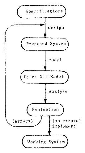
Figure 1. One use for Petri nets in the design, evaluation, and implementation of systems.
Once a Petri net model of a system (existing or proposed) has been created, it can be simulated and analyzed. The analysis of a Petri net can uncover possible problems with the modelled system, leading to a revision to correct the problems and produce a better system. This process can be iterated until the Petri net analysis indicates that no further problems exist in the model. One goal of the work with Petri nets is to develop the theory to a point where the specification, design, analysis, evaluation and implementation of a new system can be done completely in terms of Petri nets.
The motivation for the theory of Petri nets, then, is to develop techniques for the modeling and analysis of systems which exhibit concurrency. Current work has focused to a large degree on computer hardware and software systems. To show what is currently possible with Petri nets, we first give an informal definition of Petri nets and then consider analysis techniques.
A Petri net can be defined in many ways.
However, the most common representation of a Petri net is as a graph.
A Petri net graph has two types of nodes: places and transitions.
Places are connected to transitions (and vice versa) by directed arcs.
Thus, a Petri net graph can be defined as a triple (T,P,A) where,
T = {t1,t2,...,tm} is a set of transitions,
P = {p1,p2,...,pn} is a set of places, and
A ⊆ (PxT) ∪ (TxP) is a set of arcs.
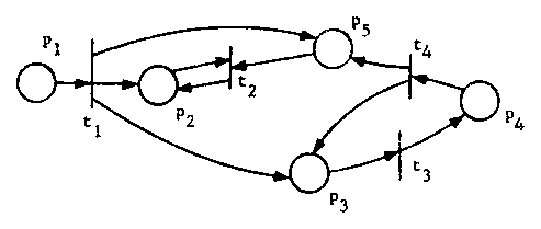
Figure 2. A Petri net.
The dynamic behavior of a Petri net is controlled by tokens.
Tokens reside in the places of a Petri net, and are represented by
small black dots in the circles representing the places. Several
tokens may reside in a place at a time.
A marking, μ, is an assignment of tokens to places, and is
represented by a vector μ = (μ1,μ2,μ3,...,μn).
The ith component of the marking, μi, defines the number of
tokens in the ith place, pi.
Figure 3 shows a marking μ = (1,0,2,0,0)
for the Petri net of Figure 2.
A marking defines the current
state of the Petri net.
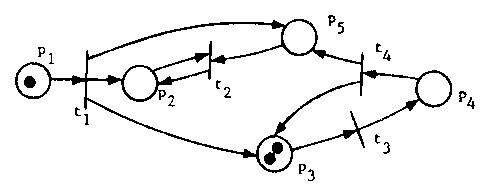
Figure 3. A marked Petri net.
A Petri net is executed by firing transitions. A transition
is enabled if all of its input places have tokens. An enabled
transition may fire by removing one token from each of its input
places and depositing one token in each of its output places. This
produces a new marking for the Petri net.
Figure 4 shows the marking which results from firing transition t1 in
the marked Petri net of Figure 3.
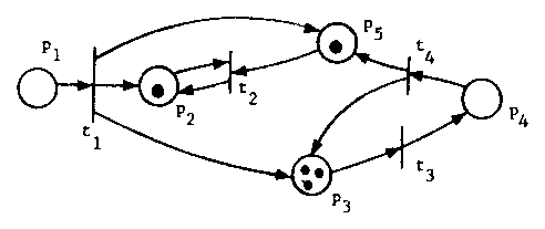
Figure 4. The marked Petri net which results from firing transition t1 in Figure 3.
Starting in an initial marking μ0, an enabled transition tj1 can be fired leading to a new marking μ1. This marking may enable another transition tj2 which can be fired leading to the marking μ2. Firing a transition tj3 in μ2 will lead to marking μ3. This can continue as long as there is an enabled transition in the current marking. The sequence of transition firings, tj1, tj2, tj3, ... defines an execution of the Petri net with initial marking μ0. For the Petri net of Figure 4, with the marking shown, one execution sequence is t3, t2, t4, t3, t3, t2, t4, t4, t3, ...
The set of all markings which can result from legal firing sequences, for a Petri net C = (T,P,A) and an initial marking μ0 is its reachability set, R(C,μ0). A marking μ is reachable from μ' if there is any sequence of transition firings which will lead from μ to μ'. A marking is always reachable from itself. The reachability set is the set of all reachable markings from an initial marking.
In general, a Petri net defines a set of transitions which are enabled in the current marking. If this set is empty, the execution of the Petri net halts. If the set has exactly one element, then this transition must eventually fire. However, if several transitions are enabled, then a choice must be made as to which will fire next. The choice can be made randomly or by controlled by some external force, depending upon the semantics of the system represented by the Petri net. There are two special cases which are of interest, however.
If two transitions are enabled, and their inputs are disjoint,
then the two transitions are concurrent (Figure 5). The
representation of this concurrency allows either transition to fire,
so all possible interleavings of the concurrent transitions
are possible. If the transitions do not have disjoint inputs,
then firing one may disable the other.
These transitions are in conflict (Figure 6). Conflict means
that only one of the conflicting transitions may fire; a
decision must be made as to which will fire.
The concepts of concurrency and conflict are central to Petri net
theory.
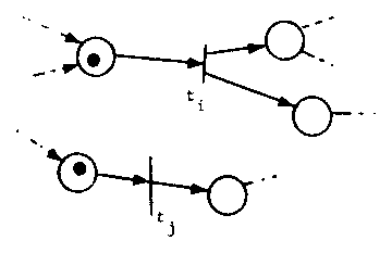
Figure 5. Concurrency in transition firing. Transitions ti and tj are concurrent.
Figure 6. Conflict in transition firing. Transitions ti and tj are in conflict.
To be useful as a model of parallel computation, we must be able to analyze Petri nets, to determine properties of the modeled system. Part of the problem here is that the development of algorithms to determine properties of Petri nets depends upon the properties to be determined. Thus, the approach taken by most researchers has been to choose properties which appear to be useful and investigate them. This is not to say that other properties cannot be analyzed, simply that no one may have considered them yet.
An example of a problem which has received considerable attention is the liveness problem. A Petri net is live if a deadlock cannot occur. This problem has been motivated by the modeling of operating systems. Resource allocation in an operating system sometimes leads to deadlock, where one process has a resource, q, and is waiting for a resource r, and another process has r and is waiting for q. A deadlock in a Petri net would be reflected as a transition which cannot fire (is not enabled), and no sequence of transition firings will take the net to a marking which allows it to fire. A Petri net is live if there is no deadlock. This implies that for all markings, μ, in the reachability set, and for all transitions tj, there exists a sequence of transitions leading from μ to some marking μ' in which tj is enabled.
The other approach taken has been to develop general tools for
the analysis of Petri nets. When a new property is to be investigated,
these general tools can be used, if the new property can be cast in
the terms of the general technique. The major tool along these
lines is the reachability set.
The reachability set of a marked Petri net is the set of all
markings which can result from legal firing sequences.
This set is, in general, infinite.
What is desired is a finite representation of this set.
Then many analysis questions may be solved by an examination
of the reachability set.
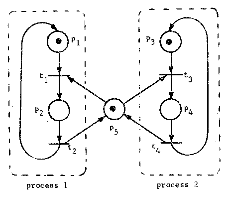
Figure 7. A Petri net model of the mutual exclusion problem for two processes. Places p2 and p4 represent activity which cannot occur at the same time.
As an example of the use of the reachability tree for analysis, consider the Petri net of Figure 7. This Petri net models the mutual exclusion problem: places p2 and p4 represent the updating of a data base shared between processes 1 and 2; both processes cannot update the data base at the same time. For correctness, we must show that no reachable marking has p2 = 1 and p4 = 1, simultaneously.
The reachability tree is a finite representation of the reachability set. The tree is formed by using the initial marking as the root. For each enabled transition, a branch is created from the initial marking to the marking which results from firing the enabled transition. For each of the new markings which are added to the tree because of these firings, we repeat the process, adding branches from a marking for each transition enabled in that marking to the new marking which results from firing the enabled transition. This process would produce an infinite reachability tree. To make the tree finite two rules are used. First, if a marking is generated which has already been generated, no successors are generated for this duplicate marking. All the successor markings from this duplicate marking will have been generated from the previous marking.
Second, if a marking μ is generated which is greater
than some marking μ' on the path from the root to μ
(so μ' is an ancestor of μ and μ > μ'), then the components
of μ which are greater than the corresponding components of
μ' are replaced by ω. The symbol ω acts like "infinity".
The idea here is that a sequence of transition firings, σ, took
the Petri net from marking μ' to marking μ. But since μ > μ',
the sequence σ is again legal from μ. If we repeat the sequence
σ, the components of μ which are greater than the corresponding
components of μ' will get larger and larger. By repeating the
sequence σ often enough, we can make these components of the marking
arbitrarily large. Figure 8 illustrates the reachability tree for
a simple Petri net.
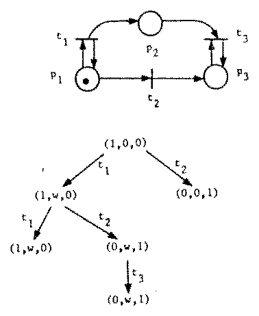
Figure 8. A Petri net and its reachability tree.
The reachability tree can be used to solve several problems for Petri nets. For example, a Petri net is k-safe if the number of tokens in a place never exceeds k. This is necessary if the Petri net were to be directly implemented: a place could be represented by a hardware counter for 0 to k. A Petri net is bounded if all places are k-safe for some k. To test for a bounded net, simply construct the reachability tree; if ω occurs in the tree, then the net is not bounded. If the net is bounded, the bound for each place can be determined by inspection. Other similar problems can be solved by the reachability tree.
Another analysis question is the reachability problem. This question is posed as: Given a marked Petri net, and a marking μ, is μ in the reachability set of the marked Petri net (i.e., is it possible to get into the marking μ from the initial marking)? This problem cannot, in general, be answered by the reachability tree (although we can determine if some marking μ' > μ is reachable). This problem is very important, however, since many analysis questions can be posed as reachability problems. The liveness problem, for example, can be converted into a reachability problem [2].
Another approach can be used for the reachability problem. A matrix,
D, can be defined, where each row represents a transition and each
column, a place. The element D[j,i] represents the change in
the marking in place pi when transition tj is
fired. If ej is an m-vector with zeros everywhere except
the jth position which is one, then μ + ej*D
is the marking resulting from firing transition tj in
marking μ. This means that if a marking μ' is reachable from
μ, then the equation
(1) μ' = μ + f*D
Unfortunately, the existence of the f vector in equation (1) above is a necessary, but not sufficient condition for reachability. Thus, if f does not exist (as a vector of nonnegative integers), then μ' is not reachable from μ, but if f does exist, μ' still need not be reachable from μ. Figure 9 is an example of this situation. The marking (0,0,0,1) is not reachable from (1,0,0,0) although a firing vector, f = (1,1) exists.
Recent results seem to indicate that the reachability problem
is solvable [3], but it is extremely hard [4]. Thus although the problem
can be solved, it may take much too much time and money to be
worthwhile, in general. Other problems, such as the equality of
the reachability sets of two Petri nets (useful for considering equivalence
and optimization) are known to be unsolvable [5]. This would seem
to severely limit the usefulness of Petri nets for modeling and
analysis.
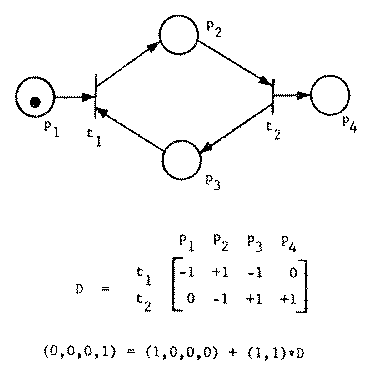
Figure 9. An example showing that the existence of a firing vector is not sufficient for reachability.
The decidability problems of Petri nets are emphasized by those studies which have tried to extend Petri nets to be a more powerful modeling tool. Many extensions, such as allowing multiple arcs between the places and transitions, can be shown to be equivalent to non-extended Petri nets [6]. Other extensions, such as introducing inhibitor arcs (transition can fire only if inhibitor places have zero tokens), priorities between transitions (to decide which transition fires first), timings, and so on result in a model which is equivalent to a Turing machine [7]. Thus, essentially all analysis questions become undecidable.
Two alternative approaches to the analysis problem of Petri nets are being considered. One is to restrict Petri net synthesis to produce Petri nets which are correct due to their construction [8]. Another approach is to consider only restricted subclasses of Petri nets.
Several subclasses of Petri nets have been identified and studied. Finite state machines are easily shown to be equivalent to a subclass of Petri nets. A finite state machine Petri net has only one input and one output for each transition.
Marked graphs are another common subclass of Petri nets. Every place in a marked graph is restricted to being an input of exactly one transition and an output of exactly one transition (Figure 10). This eliminates sharing of places between transitions and so eliminates conflict. Marked graphs are therefore of limited modeling power, but have been throughly investigated [9] and are well understood.
A slightly more general class of Petri nets, free choice nets,
which restrict conflicting transitions to have identical
inputs have also been investigated [10].
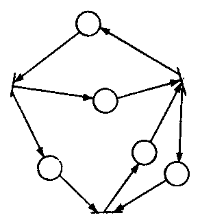
Figure 10. A marked graph. Each place is an input and output to only one place.
Petri nets have been receiving increased attention as a model of parallel computation. In large part this is due to the simplicity of the Petri net model coupled with a careful balance of modeling power and decision power. The modeling power of Petri nets is quite good, as witnessed by the wide variety of systems which can be modelled by Petri nets. The decision power is also good, since the reachability problem is decidable, and most problems can be converted into reachability problems. Subclasses of Petri nets increase the decision power, but at a cost of being unable to model a large number of systems. Extended Petri net models increase the modeling power, but in all known cases at the expense of decision power, since most analysis questions become undecidable.
We would expect the use of Petri nets to increase for the near future.
This paper is meant to be only a brief introduction to Petri
nets. Further information can be obtained from the other papers
presented in this session. Also, several other papers might be of
interest. A more extensive survey can be found in [11].
Other important papers include [12, 13, 14, 15, 16, 17].
| Home | Comments? |