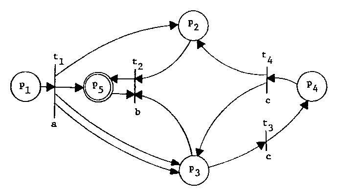
Figure 2. Graphical representation of the Petri net of Figure 1.
| Home | Up | Questions? |
A class of automata based upon generalized Petri nets is introduced and defined. The language which a Petri net generates during an execution is called a computation sequence set (CSS). The class of CSS languages is shown to be closed under union, intersection, concatenation, and concurrency. All regular languages and all bounded context-free languages are CSS, while all CSS are context-sensitive. Not all CSS languages are context-free, nor are all context-free languages CSS. Decidability problems for CSS hinge on the emptiness problem for CSS. This problem is equivalent to the reachability problem for vector addition systems, and is open.
Petri nets have been used by several researchers for the description and analysis of systems of parallel processes [8, 9, 16, 17, 18]. Although the majority of current research with Petri nets is still directed toward parallel computation, in this paper we consider Petri nets as an automaton in the same way as finite state machines, pushdown stack automata, and Turing machines. Viewed in this way, a language can be naturally associated with the execution of a Petri net. Consideration of the properties of the class of languages generated by Petri nets yields both new properties of Petri nets and an interesting addition to formal language theory.
We first define the new class of automata based on Petri nets. Then, the language of a Petri net, called a computation sequence set (CSS), is defined. A computation sequence set contains all possible computation sequences which may represent an execution of a Petri net from its start state to a final state. Formal definitions of these concepts are given in Section 2. Section 3 investigates the closure properties of the class of computation sequence sets, and Section 4 relates this new class of languages to the classical hierarchy of regular, context-free, context-sensitive, and type-0 languages. Section 5 then considers some decidability questions and conclusions about CSS as a class of languages.
We begin by giving a definition for the class of Petri nets. This definition follows the approach of [17] and is essentially the same as the Generalized Petri Nets of [6] although different notation is used. This general definition subsumes, or is equivalent to, most other definitions of Petri nets.
A Petri net, C, is a 5-tuple defined by
where
Each transition, tj ∈ T, is an ordered triple defined by
(The Appendix gives a brief summary of the theory and notation of bags. Bags are essentially an extension of sets which allow multiple occurrences of an element in a bag. The number of occurrences of an element x in a bag β is given by the function #(x, β). Our use of bags is for descriptive purposes, so we use the notation and concepts of set theory with which the reader should be familiar. For a more complete development of bag theory, the reader is referred to [2].)
The sets P, T, Σ are assumed to be finite. The cardinality of the set P is n and of the set T, m. Arbitrary elements of P and T are denoted by pk (1 ≤ k ≤ n) and tj (1 ≤ j ≤ m), respectively. The set Σ is not generally defined explicitly since it can be inferred from the definitions of the transitions (Σ = {σj | (σj, Ij, Oj) ∈ T}). We use σ, σj and early lowercase Roman letters (a, b, c,...) to represent elements of Σ.
An example Petri net is defined in Figure 1.
| C | = | (P, T, Σ, S, F) |
| P | = | {p1, p2, p3, p4, p5} |
| T | = | {t1, t2, t3, t4} |
| Σ | = | {a, b, c} |
| S | = | p1 |
| F | = | {p5} |
| t1 | = | (a, {p1}, {p2, p3, p3, p5}) |
| t2 | = | (b, {p2, p3, p5}, {p5}) |
| t3 | = | (c, {p3}, {p4}) |
| t4 | = | (c, {p4}, {p2, p3}) |
Figure 1. Definition of an example Petri net.
When working with Petri nets, we need to refer to the separate components of the ordered triples which define the transitions. To allow us to specify easily the portion of a transition which we are discussing, we define three projection functions -- the label function (σ), the input function (I), and the output function (O). For a transition tj = (σj, Ij, Oj), these functions are defined by
| σ(tj) | = | σj |
| I(tj) | = | Ij |
| O(tj) | = | Oj |
To map sequences of transitions into sequences of symbols, we extend the label function by
| σ(x) | = | ε | if x | = | ε, | |
| σ(x) | = | σ(tj)σ(y) | if x | = | tjy, tj ∈ T, y ∈ T*. |
(We use ε to denote the empty sequence. Σ* denotes the set of all strings over an alphabet Σ.)
A convenient visual representation of a Petri net is a bipartite directed graph. Both places and transitions are represented as nodes in the graph. To distinguish them, places are represented by circles and transitions by bars. An arc is directed from a transition tj to a place pk for each occurrence of pk in the output bag, O(tj), of the transition. An arc is directed from a place pk to a transition tj for each occurrence of pk in the input bag, I(tj), of tj. Since the ordering of places and transitions is unimportant, the start place is assumed to be p1. Final places are indicated by a circle around the node representing them. The Petri net of Figure 1 is graphed in Figure 2.
Figure 2. Graphical representation of the Petri net of Figure 1.
The graph representation of a Petri net contains all the information which is necessary to define the net. Thus we give graph representations of Petri nets rather than formal definitions for our illustrations.
The above definitions are concerned with the description of the structural properties of a Petri net. Since the Petri net is an abstract machine, it also has computational properties. The computational properties refer to its behavior during an execution. The execution of a Petri net is directed by the existence and location of tokens in the net. Tokens are abstract entities which we represent by black dots in the circles of the graphical representation of a Petri net. Tokens move about the Petri net in a manner dictated by the execution rules for Petri nets. These rules are
A transition is enabled if all of its input places have (a sufficient number of) tokens in them. A transition fires by removing tokens from all of its input places and placing tokens in all of its output places. These definitions are made more precise by
Execution of a Petri net begins with one token in the start place. Each time that a transition fires, it may change the number and/or location of tokens in the Petri net and therefore the state of the net. A Petri net may halt whenever it reaches a final state (one token in a final place and zero tokens elsewhere) or it may continue execution. If the set, U, of enabled transitions is empty, the Petri net must halt.
Figure 3 illustrates the concept of the execution of a Petri net by using the graphical representation of Figure 2 to present one possible execution. At each step, the Petri net and its tokens are given as well as the set U of enabled transitions and the selected transition which fires.
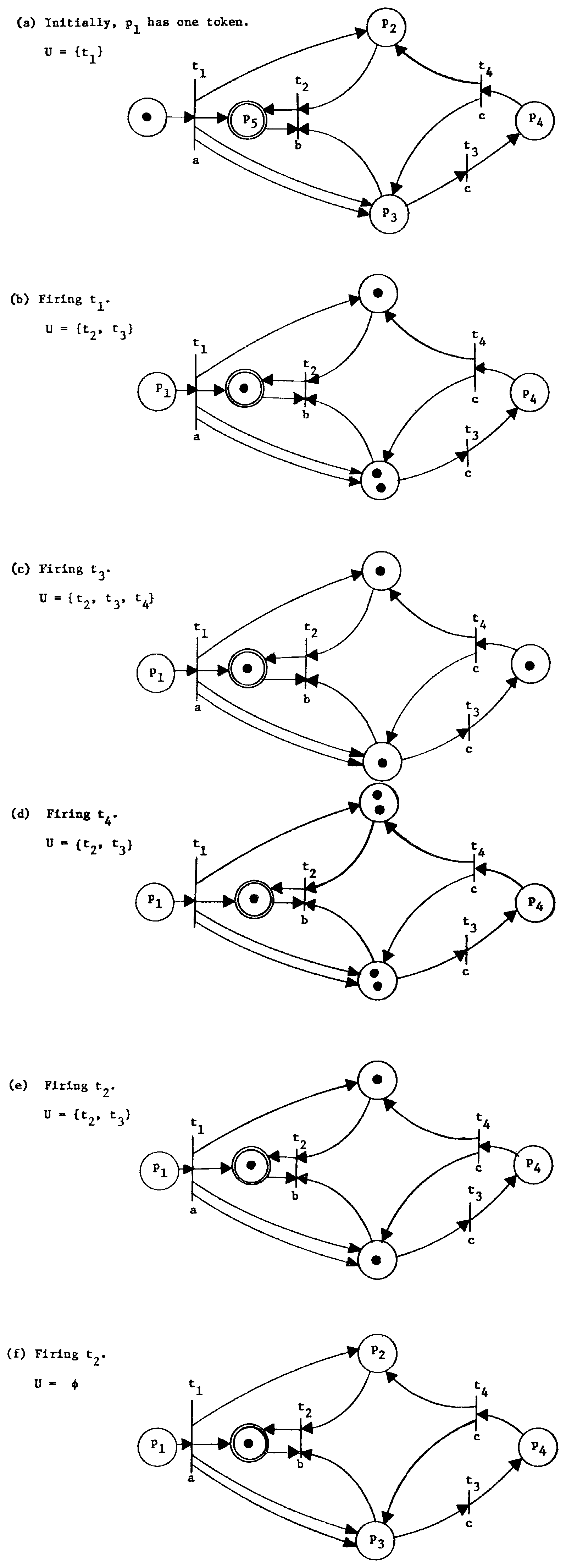
Figure 3. One possible execution of the Petri net of Figure 1.
The state of a Petri net is defined by the number and location of tokens in the net. This can also be expressed as the number of tokens (possibly zero) in each place of the net and is commonly called a marking. The number of tokens in each place will always be a nonnegative integer number, and we represent the state of a Petri net by an n-vector of nonnegative integers. The firing of a transition represents a change in the state of the Petri net. A state is reachable if there exists some sequence of firings which transforms the start state (the state associated with one token in the start place and zero tokens elsewhere) into the desired state.
We define Q to be the reachable state space of a Petri net. Q is also called the marking class of a Petri net. If N represents the set of nonnegative integers then Q ⊆ Nn. Each element of Q is an n-vector whose kth component represents the number of tokens in place pk (1 ≤ k ≤ n). We denote by S both the start place and the vector (1, 0, 0,...); F denotes both the set of final places and the set of vectors representing one token in a final place and zero tokens elsewhere (the final states).
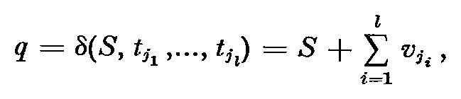
The next-state function, δ, is a (partial) function from Nn × T into Nn. For a state vector, q, and a transition, tj, the next-state function, δ(q, tj), is defined if and only if for all k, 1 ≤ k ≤ n,
Thus a transition tj is enabled in a state q if and only if δ(q,tj) is defined. If δ(q, tj) is defined, then the new state vector defined is the state resulting from the firing of tj. The kth component of the new state is defined by
Since qk ≥ #(pk,I(tj)) if δ(q,tj) is defined and #(pk,O(tj)) ≥ 0, we see that if δ(q,tj) is defined, then δ(q,tj) ≥ 0 and hence δ(q, tj) ∈ Nn.
The definition of δ(q,tj) can be recast as a vector replacement system [12]. We specify, for each transition, tj, two vectors, uj, and vj, where (uj)k = -#(pk, I(tj)) and (vj)k = -#(pk, I(tj)) + #(pk, O(tj)). Then δ(q,tj) is defined if q + uj ≥ 0, and if δ(q,tj) is defined, then δ(q,tj) = q + vj. The reachable state space of a Petri net corresponds to the reachability set of a vector replacement system (see Section 5).
As with the label function, we extend the next-state function
from a domain of individual transitions to a domain of sequences
of transitions. If x is a sequence of transitions (x ∈
T*), then
| δ(q,x) | = | q | if x = ε, | |
| = | δ(δ(q,tj),y) | if x = tjy for tj ∈ T, y ∈ T*. |
Of course δ(q,x) is defined if and only if the next-state functions of the above definition are defined for their arguments.
We can now formally define the reachable state space, Q, as the smallest subset of Nn defined by
Since we are concerned only with reachable states, we restrict the next-state function to the reachable state space, Q. Thus, δ: Q × T* → Q, and (except perhaps for the start state) the mapping is onto.
It should be clear from the definition of the state space, the next-state function, and the reachable state space that the automaton defined by (Q, δ, Σ, S, F) is equivalent to (P, T, Σ, S, F) as a mathematical formulation of a Petri Net. We use both definitions interchangably,
Each separate execution of a Petri net defines, or is defined by, the sequence of transitions which are fired during the execution of the net. We say that a sequence of transitions, x ∈ T*, is legal if it represents a possible sequence of transition firings from the start state, S. Thus a sequence is legal if δ(S, x) is defined. A sequence is complete if it is legal and δ(S, x) ∈ F.
To illustrate these concepts, consider the execution shown in
Figure 3. This execution is completely defined by the transition
sequence t1t3t4t2t2. For this example, the sequence is both
legal and complete. The sequences t1t3t4 and
t1t3t3t4t4t2t2 are legal but not complete, since
| δ(S, t1t3t4) | = | (0,2,2,0,1), |
| δ(S, t1t3t3t4t4t2t2) | = | (0,1,0,0,1), |
The sequences t1t4, t2t3t3t4, and t4 are neither complete nor legal.
Associated with each sequence of transitions, x ∈ T*, is the sequence of symbols, y ∈ Σ*, defined by y = σ(x). A sequence of symbols which corresponds to a legal and complete transition sequence is a computation sequence. Each computation sequence represents one (or more than one) execution of the Petri net which begins with one token in the start place and ends with one token in a final place, while all other places have zero tokens both before and after the execution (although probably not during the execution). The computation sequence set of a Petri net is the set of all computation sequences for that net. We denote the computation sequence set of a Petri net, C, by L(C). Formally,
Many Petri nets may generate the same CSS. We define two Petri nets to be equivalent if their CSS are equal. The CSS is the language of the Petri net and is considered the characterizing feature of the net.
The next-state function is again extended to be defined over computation sequences as well as transition sequences by defining δ(q, y) = q' for any string y ∈ Σ* for which there exists a transition sequence, x ∈ T*, with y = σ(x) and δ(q, x) = q'. Note that with this definition δ may no longer be single-valued, but may yield a set of states. If δ is not single-valued, then the Petri net is nondeterministic. We define a CSS to be nondeterministic if every Petri net which generates it is nondeterministic. A deterministic CSS is then a CSS for which there exists a deterministic Petri net which generates it. Figure 4 is a nondeterministic Petri net with a nondeterministic CSS.
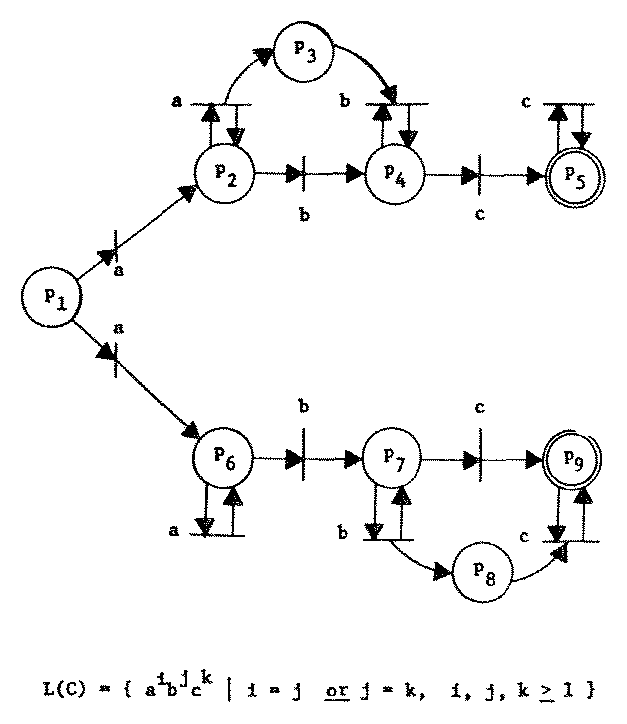
Figure 4. An inherently nondeterministic Petri net.
(The proof that no equivalent Petri net is deterministic is similar to the proof in [4] that this CSS is an inherently nondeterministic context-free language.)
Having defined the Petri net automaton and its associated language, we turn now to investigating the properties of the class of CSS languages. We begin our investigation by considering the closure properties of CSS under union, intersection, concatenation, and concurrent composition. We first define a restricted class of Petri nets whose special properties are convenient in the proofs of closure under these forms of composition.

Figure 5. A "pathological" Petri net.
The general definition of Petri nets in Section 2 allows the construction of "pathological" Petri nets, such as the net of Figure 5, whose strange properties make the proofs which follow unnecessarily complicated. In particular, the transitions with empty input or output bags require special attention. We avoid these problems by showing that such transitions can be eliminated without changing the language of the Petri net. This is done by introducing a new place, pr, to the net. This place is made an input and output to every transition in the net. As long as there is a token in this place, the possible transition sequences are identical to the transition sequences of the original net; when this token is removed, all transitions are disabled. Using this approach we introduce a new start place S' and final place, pf. New transitions are added which mimic the old transitions except that the first transition to fire places a token in pr, and the last transition to fire removes this token. From this construction, we define a restricted class of Petri nets in standard form by
DEFINITION. A Petri net, C = (P, T, Σ, S, F) is in standard form if
A Petri net in standard form has no transitions with empty input or output bags. It also has a start place which is an output of no transition and a special "final" place which is an input to no transition.
The execution of a Petri net in standard form starts with one token in the start place. The first transition removes this token and after this firing the start place is always empty. Eventually (if the transition sequence is complete) a token is placed in the final place. This token cannot be removed from the final place both because no transition has an input from the final place and because all transitions are disabled. The restrictive nature of the standard form Petri nets is useful when defining compositions of Petri nets. To show that standard form Petri nets are not less powerful than general Petri nets, we prove the following theorem.
Theorem 1. Every Petri net is equivalent to a Petri net in standard form.
Let C = (P, T, Σ, S, F) be a Petri net.
Define C' = (P', T', Σ, S', F') by
| P' | = | P ∪ {S', pr, pf}, | where {S', pr, pf} ∩ P = ∅, | |
| F' | = | {S',pf} | if S ∈ F, | |
| = | {pf} | if S ∉ F. |
We define four kinds of transitions in the set T'. First, for all
tj ∈ T, we include a transition tj' = (σ(tj), I(tj) + {pr}, O(tj)
+ {pr}) in T'. To start the net we consider that two kinds of
transitions in T could fire first; those with I(tj) = {S} and
those with I(tj) = ∅. For each of these we define tj'' by
| tj'' | = | (σ(tj), {S'}, O(tj) + {S, pr}) | if I(tj) = ∅ , | |
| = | (σ(tj), {S'}, O(tj) + {pr}) | if I(tj) = {S}. |
Similarly the last transition to fire could be either a
transition with O(tj) = ∅ or O(tj) = {pk} such that
pk ∈ F. For each of these we define tj''' by
| tj''' | = | (σ(tj), {pr} + I(tj), {pf}) |
These transitions define a legal and complete transition sequence
| tj1'' tj2' tj3' ... tjl-1' tjl''' (l > 2) |
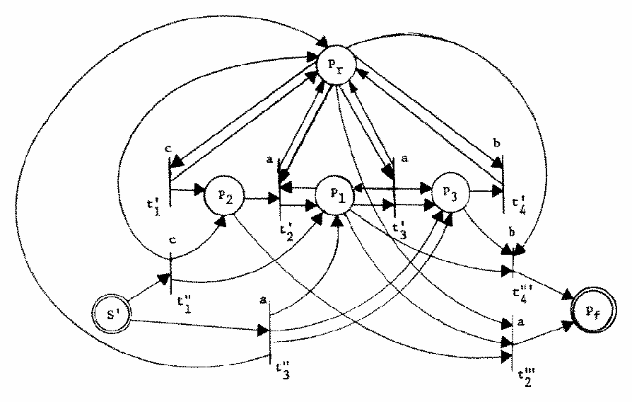
Figure 6. A standard form Petri net equivalent to the Petri net of Figure 5.
We consider two CSS L1 and L2 and two Petri nets in standard form, C1 = (P1, T1, Σ, S1, F1) and C2 = (P2, T2, Σ, S2, F2) with L1 = L(C1) and L2 = L(C2). We construct a new Petri net, C' = (P', T', Σ, S', F') whose language, L' = L(C'), is the desired composition of L1 and L2. Figure 7 gives example Petri nets for C1 and C2 which we use in our discussions to illustrate the construction of C'.
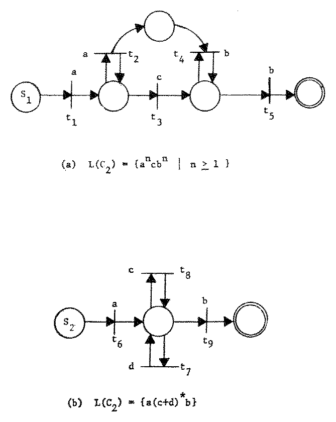
Figure 7. Illustration Petri nets.
The concatenation of two languages can be formally expressed as
| L1L2 | = | {x1x2 | x1 ∈ L1 and x2 ∈ L2}. |
Theorem 2. If L1 and L2 are CSS, then the concatenation of L1 and L2 is CSS.
We define a Petri net, C' = (P', T', Σ, S', F'), where
| P' | = | P1 ∪ P2, | ||||||
| T' | = | T1 ∪ T2 ∪ {(σj, {pf}, Oj) | (σj, {S2}, Oj) ∈ T2, pf ∈ F1}, | ||||||
| S' | = | S1, | ||||||
| F' | = |
|
With this definition we have overlapped the final places of C1 with the start place of C2. The transition which signals the termination of C1 by placing a token in an element of F1 acts to initiate C2 by placing a token in a place equivalent to S2. Since both nets are in standard form, all transitions of the C1 subnet are disabled when the token is placed in a final place of F1, and all transitions of the C2 subnet are disabled until a token is placed in one of these places. Any "extra" tokens produced by an execution of the C1 subnet remain in that net after the token is placed in an element of F1, so that C' cannot reach a final state unless both C1 and C2 have reached final substates. Thus, if a sentence is generated by C', it must be composed of a sentence which was generated by C1 followed by a sentence generated by C2, and is in the concatenation of L1 and L2. Similarly, any computation sequence in the concatenation has a path from S1 to an element of F2 in C', and is an element of L'. This shows that CSS are closed under concatenation. Figure 8 illustrates this construction.
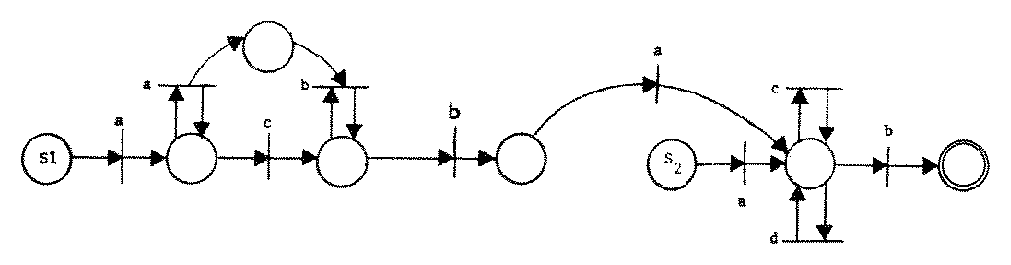
Figure 8. A Petri net whose CSS is the concatenation of the Petri nets of Figure 7.
Since languages are sets of strings, a common method of
composition is to take the union of two languages. This is
defined as
| L1 ∪ L2 | = | { x | x ∈ L1 or x ∈ L2}. |
Theorem 3. If L1 and L2 are CSS, then the union of L1 and L2 is CSS.
We construct C' with L(C') = L1 ∪ L2. The definition of C' is
| P' | = | P1 ∪ P2 ∪ {S'}, | ||||||
| T' | = | T1 ∪ T2 ∪ {(σj, {S'}, Oj) | (σj, {S1}, Oj) ∈ T1 or (σj, {S2}, Oj) ∈ T2}, | ||||||
| S' | = | S1, | ||||||
| F' | = |
|
This construction introduces one new start place and transitions which make this new start place equivalent to both S1 and S2. Placing the start token in S' enables a transition corresponding to every transition which would be enabled by placing a start token in S1 or S2. When one of these transitions fires, the output tokens are placed in a subnet defined by (P1, T1) or (P2, T2) and execution continues exactly as it would in C1 or C2. The null sequence is included by the definition of F'. This construction generates L1 ∪ L2. Thus CSS are closed under union. The construction of C' from C1 and C2 is illustrated in Figure 9 for the C1 and C2 of Figure 7.
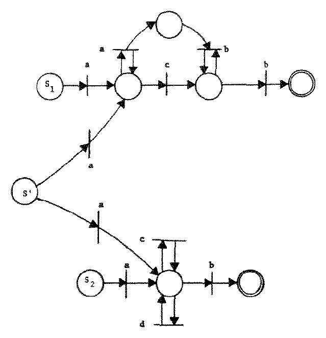
Figure 9. A Petri net whose CSS is the union of the CSS of the Petri nets of Figure 7.
As with union, the intersection composition is similar to the set
theory definition of intersection and is given for CSS by
| L1 ∩ L2 | = | { x | x ∈ L1 and x ∈ L2}. |
Theorem 4. If L1 and L2 are CSS, then the intersection of L1 and L2 is CSS.
The construction of a Petri net to generate the intersection of two CSS is rather complex. At a given point in a computation sequence if a transition fires in one Petri net, there must be a transition in the other Petri net with the same label which can fire also. When there exists more than one transition in each Petri net with the same label, we consider all possible pairs of transitions from the two nets. For each of these pairs, we create a new transition which can fire if and only if both transitions in the old nets can fire. This is done by making the input (output) bag of the new transition the bag sum of the input (output) bags of the pair of transitions from the old Petri nets. Thus if tj ∈ T1 and tk ∈ T2 are such that σ(tj) = σ(tk) = σjk, then we have a transition tjk = (σjk, Ij + Ik, Oj + Ok) in T'. Some of these transitions will have inputs which include the start place. If for a transition tjk in T' as defined above, I(tjk) = {S1, S2}, then we add a transition t'jk with I(t'jk) = {S'}, and other components equal. Similarly, for any transition tjk with O(tjk) = {pf1, pf2} with pf1 ∈ F1 and pf2 ∈ F2, we add a new transition t''jk which is equal to tjk except that O(t''jk) = {pf'}. F' is {pf', S'} if S1 ∈ F1 and S2 ∈ F2 and {pf'} otherwise. Figure 10 illustrates this construction.
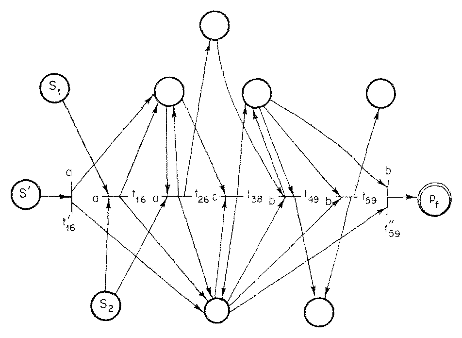
Figure 10. A Petri net whose CSS is the intersection of the CSS of the Petri nets of Figure 7.
Concurrent composition allows all possible interleavings of a computation sequence from one CSS with a computation sequence from another CSS. Riddle [19] has introduced the Δ operator to represent this concurrency. The concurrency operator has also been called the "shuffle" operator [5]. It is defined for two strings by
where a, b ∈ Σ, and x1, x2 ∈ Σ*. The
concurrent composition of two languages is then
| L1 Δ L2 | = | {x1 Δ x2 | x1 ∈ L1 and x2 ∈ L2}. |
For example, ab Δ c = abc + acb + cab, (a + b) Δ c = ac + ca + bc + cb. (The shuffle operator was defined so that it appears that strict alternation of elements of two strings is required. That is, if x = x1x2... xk and y = y1y2 ... yk, then shuffle(x,y) = x1y1x2y2 ... xkyk. However, xi and yi are allowed to be (possible null) strings, not simply elements, of the alphabet.)
It is easily shown that regular, context-sensitive and type-0 languages are closed under concurrency, while context-free languages are not. For CSS, we have
Theorem 5. If L1 and L2 are CSS, then the concurrent composition of L1 and L2 is CSS.
The construction of a Petri net to generate the concurrent
composition of L1 and L2 given nets to generate these CSS is
basically the construction of a Petri net which places tokens in
both the start places of C1 and C2, and then accepts the
input if tokens are in any two final places (one from each net),
and no other places. To start the combined Petri net we
introduce a new start place, S'. The first transition which
fires in the concurrent composition of two CSS will come from
either C1 or C2. If the first transition which
fires is from C1, then we modify it to also place a
token in S2, allowing the Petri net C2 to then start
whenever it wishes. A similar strategy is used if the first
transition is from C2. Thus C' is defined by
| P' | = | P1 ∪ P2 ∪ {S', pf'}, |
| T' | = | T1 ∪ T2 ∪ TSF, |
| F' | = | {pf'}, |
where,
| TSF | = | {(σj, {S'}, Oj + {S2}) | (σj, {S1}, Oj) ∈ T1} |
| ∪ | {(σj, {S'}, Oj + {S1}) | (σj, {S2}, Oj) ∈ T2} | |
| ∪ | {(σj, Ij + {pk}, {pf'}) | (σj, Ij, {pf}) ∈ T1, pf ∈ F1, pk ∈ F2} | |
| ∪ | {(σj, Ij + {pk}, {pf'}) | (σj, Ij, {pf}) ∈ T2, pf ∈ F2, pk ∈ F1} |
The last two types of transitions added to T' by TSF remove the tokens from final places in C1 and C2 and place them in a new final place when the last transition of the composition is fired. This construction is demonstrated in Figure 11.
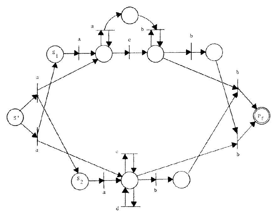
Figure 11. A Petri net whose CSS is the concurrent composition of the CSS of the Petri nets of Figure 7.
The construction is correct only for ε-free CSS. However, if L1 = {ε} ∪ L1+ with ε ∉ L1+, then L1 Δ L2 = L2 ∪ (L1+ Δ L2). Thus, since CSS are closed under union, CSS are closed under concurrent composition.
The closure properties of CSS under many other operations can be investigated, but for our purposes the above four are most relevant. It is easily shown that CSS are also closed under reversal, ε-free homomorphism, and ε-free regular substitution [17]. Hack has shown that CSS are closed under ε-free homomorphism, ε-free Finite State Transducer mappings, and inverse homomorphisms. He has also shown that CSS are not closed under Kleene star or general substitution [7].
It is conjectured that CSS are not closed under complement.
Hopcroft and Ullman [10] have compiled a table of closure properties of regular, context-free, context-sensitive, and type-0 languages for several closure operations. A similar study for CSS as a class of languages might shed some further light on the character of the CSS languages and indirectly, on their relationship to these other classes of languages. Knowledge of the relationship between CSS languages and these other classes of languages might be useful for establishing decidability results for CSS from the known results for these languages.
Thus, we turn now to investigating the relationship between CSS and the classes of regular, context-free, and context-sensitive languages.
One of the simplest and most studied classes of formal languages is the class of regular languages. These languages are generated by regular grammars and finite state machines. They can be characterized by regular expressions. Problems of equivalence or inclusion between two regular languages are decidable and algorithms exist for their solution [10]. With such a desirable set of properties it is encouraging that we have the following theorem.
Theorem 6. Every regular language is CSS.
The proof of this theorem is based on the fact that every regular
language is generated by some finite state machine. A finite
state machine is defined as a 5-tuple, (Q, δ, Σ, S,
F), where Q is a finite state space, δ a next-state
function from Q × Σ into Q, Σ an alphabet, S
∈ Q a start state, and F ⊆ Q a set of
final states. We can construct an equivalent Petri net as
(Q, T, Σ, S, F), where the set of transitions is
| T | = | {(σi, {qj}, {qk}) | δ(qj,σi) = qk} |
This Petri net will generate the same language as the finite state machine. Thus, every regular language is CSS.
The converse to Theorem 6 is not true. Figure 7 displays a Petri net which generates the context-free language {ancbn | n ≥ 1}. Since this language is not regular, we know that not all CSS are regular. Figure 12 shows that not all CSS are context-free by exhibiting a CSS which is context-sensitive, but not context-free.
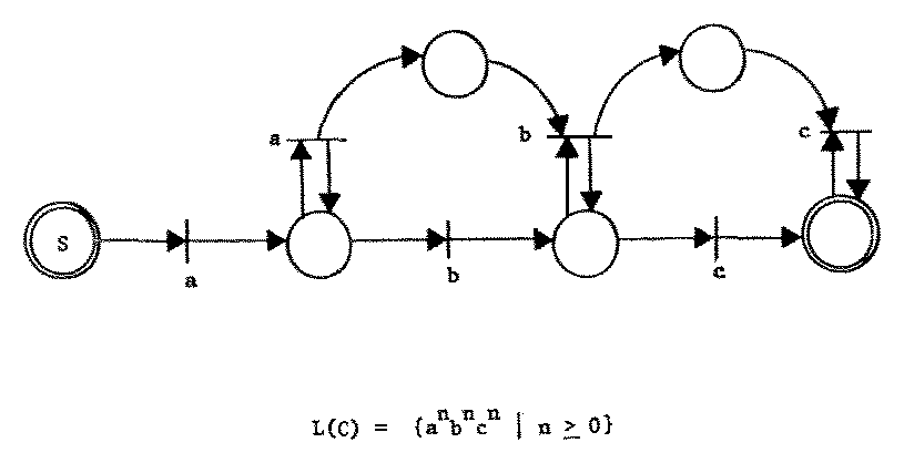
Figure 12. A context-sensitive, but not context-free CSS.
Theorem 7. There exist context-free languages which are not CSS.
Assume there exists an n-place, m-transition Petri net which
generates {wwR | w ∈ Σ*}. Let k be the number of
symbols in Σ, k > 1. For an input string xxR, let l = | x |,
the length of x. Since there are kl possible input strings x,
the Petri net must have kl distinct reachable states after l
transitions in order to remember the complete string x. If we do
not have this many states, then for some strings x1 and x2, we
have δ(S, x1) = δ(S, x2) for x1 ≠ x2. Then,
| δ(S, x1x2R) | = | δ(δ(S, x1), x2R) |
| = | δ(δ(S, x2), x2R) | |
| = | δ(S, x2x2R) | |
| = | ∈ F |
and the Petri net will incorrectly generate x1x2R,
For each transition tj, there exists a vector vj such that if δ(q, tj) is defined then δ(q, tj) = q + vj. Thus after l inputs, a Petri net will be in a state q given by
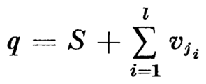
for a sequence of transitions tj1, tj2, ... tjl. Another way of expressing the above sum is
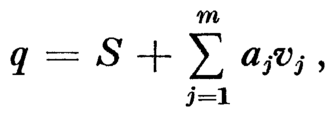
where aj is the number of times transition tj occurs in the sequence. We have also the constraint that
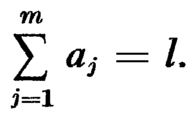
At best the vectors v1,v2, ..., vm will be linearly independent and each vector of coefficients (a1, a2, ..., am) will represent a unique state q. Since the sum of the coefficients is l, the vector of coefficients is a partition of the integer l into m parts. Knuth [13] gives the number of partitions of an integer l into m parts as
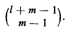
Now since
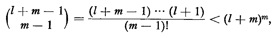
there are strictly less than (l + m)m reachable states in Q after l inputs. For large enough l, we have then that
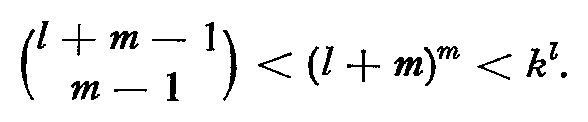
Having shown that not all context-free languages are CSS and not all CSS are context-free, the question arises, What is the class of languages which are both context-free and CSS? At present we cannot fully answer this question, but we can give an indication of some of the members of this intersection. One subset of both classes of languages is regular languages. Another subset is the set of bounded context-free languages [4].
A context-free language, L, is a bounded context-free language
over an alphabet Σ, if there exist strings w1, w2, ..., wm from
Σ* such that
| L | ⊆ | q1*w2* ... wm*. |
Ginsburg [4] has developed a detailed examination of the properties of bounded context-free languages and gives the following characterization theorem ([4, Theorem 5.4.1]).
Theorem 8. The family of bounded context-free languages is the
smallest family of sets defined by
We have already shown that every regular language (and hence every finite subset of Σ*) is CSS. We have also shown that CSS are closed under union and concatenation. Thus we have only to show that CSS are closed under the operation described in (3) above to show that bounded context-free languages are CSS,
For any case where x, y, or W is ε, xiWyi reduces to a language
of the form x*W, Wy*, x*, xiyi, or W which are CSS, for x, y
∈ Σ* and W CSS. For nonnull x and y, we define Cx
and Cy by
| x = x1x2...xk, xi ∈ Σ | y = y1y2...yl, yi ∈ Σ |
| Cx = (Px , Tx , Σ, Sx, Fx), | Cy = (Py , Ty , Σ, Sy, Fy), |
| Px = {px1,px2,...,Pxk+1}, | Py = {py1,py2,...,Pyl+1}, |
| Tx = {xi,{pxi}, {pxi+1} | 1 ≤ i ≤ k}, | Ty = {yi,{pyi}, {pyi+1} | 1 ≤ i ≤ l}, |
| Sx = px1, | Sy = py1, |
| Fx = {pxk+1}, | Fy = {pyl+1}, |
With these definitions, L(Cx) = {x} and L(Cy) = {y}. Let Cw =
(Pw, Tw, Σ, Sw, Fw) be a Petri net in standard form with
L(Cw) = W; then we define C' = (P', T', Σ, S', F') by
| P' | = | Px ∪ Py ∪ Pw ∪ {p}, |
| T' | = | Tx ∪ Ty ∪ Tw ∪ Txx ∪ TxW ∪ TWy ∪ Tyy, |
| S' | = | Sx, |
| F' | = | Fy, |
where
| Txx | = | {(xk, {pxk}, {p,px1})}, |
| TxW | = | {(σ(tj), {px1}, O(tj)) | tj ∈ TW and I(tj) = SW}, |
| TWy | = | {(σ(tj), I(t), {pyl+1}) | tj ∈ TW and O(tj) ∈ FW}, |
| Tyy | = | {(y1, {p,pyl+1}, {py2})}, |
The place p acts as a counter of the number of times that x has been generated and assures that y will be generated the same number of times if the string is correct. The additional transitions allow the proper sequencing of the Cx, Cw, and Cy nets.
With this construction, all bounded context-free languages are shown to be CSS. Are there context-free languages which are also CSS but not bounded? Unfortunately, yes. Ginsburg shows that the regular expression (a + b)* is not bounded context-free. Since this language is both context-free and CSS, we see that bounded context-free languages are a proper subset of the family of languages which are both CSS and context-free. (a + b)*canbn is both context-free and CSS but neither regular nor bounded.
We turn now to context-sensitive languages. From the example in Figure 12 we know that some CSS are context-sensitive; below we prove that all CSS are context-sensitive. Since we know that all context-free languages are also context-sensitive and there exist context-free languages which are not CSS, there exist context-sensitive languages which are not CSS. Thus the inclusion is proper.
Theorem 9. All CSS are context-sensitive.
There are two ways to show that a language is context-sensitive: Construct a context-sensitive grammar which generates it, or specify a nondeterministic linear bounded automaton which recognizes it. We use the latter technique for the proof given here. A proof using a context-sensitive grammar is given in [17].
A linear bounded automaton is similar to a Turing machine. It has a finite state control, a read/write head, and a (two-way infinite) tape. The limiting feature which distinguishes it from a Turing machine is that the amount of tape which can be used by the linear bounded automaton to recognize a given input string is bounded by a linear function of the length of the input string. In this sense it is similar to the push-down automaton used to recognize context-free languages (since the maximum length of the stack is bounded by a linear function of the input string length) except that the linear bounded automaton has random access (in the same sense as a Turing machine) to its memory, while the pushdown automaton has access to only one end of its memory.
To recognize a CSS with a linear bounded automaton, we simulate the Petri net by remembering, after each input, the number of tokens in each place. How fast can the number of tokens in a Petri net grow, as a function of the length of the input? After the transition sequence tt1 ,tt2 ,..., ttl we have seen that the Petri net is in a state defined by
where vj is the vector describing the change in state caused by
firing transition tj. Since the vj are fixed by the structure
of the Petri net, there is a maximum vector v which is
(component-wise) greater than all vj (1 ≤ j ≤ m). Thus
| q | < | S + l ⋅ v. |
If  , then the number of tokens, η, in a Petri
net after l transitions is bounded by
, then the number of tokens, η, in a Petri
net after l transitions is bounded by
| η | < | 1 + l ⋅ | v | |
Thus the number of tokens, and the amount of memory needed to remember them, is bounded by a linear function of the input length. Hence CSS can be recognized by linear bounded automata, showing that CSS are context-sensitive.
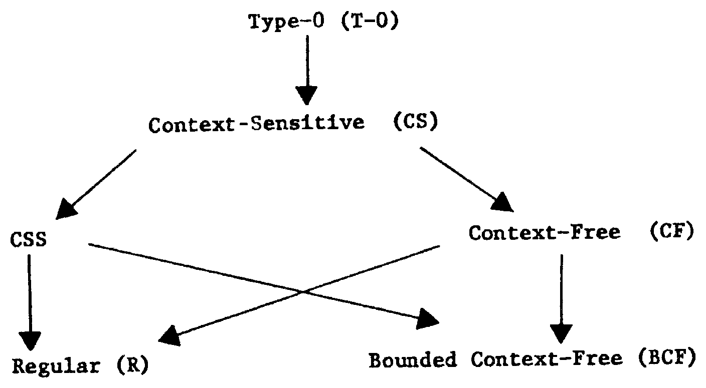
Figure 13. Relationship of CSS to other classes of languages.
Figure 13 summarizes the relationships among the classes of languages which are regular, bounded context-free, CSS, context-free, and context-sensitive. An arc between two classes of languages indicates proper containment.
A large number of problems for CSS and Petri nets are currently unanswered. The decidability of the following list of decision problems (among others) needs resolution.
The last problem above is the emptiness problem for CSS. This problem is central to the decidability properties of CSS languages. If the emptiness problem is undecidable, then all of the above questions are undecidable [17].
Another viewpoint on the emptiness problem for CSS can be obtained by considering the equivalence between the state space of the Petri net and vector replacement systems. Keller [12] has defined a vector replacement system as a triple (q0, U, V), where U and V are sets of n-vectors over the integers, with uj < vj for uj ∈ U and vj ∈ V (1 ≤ j ≤ |U| = |V|). A reachability set, Q, is defined by
(a) q0 ∈ Q.
(b) if x ∈ Q and x + uj > 0,
then x + vj ∈ Q (uj ∈ U, vj ∈ V).
Comparing this with the definition of the state space of a Petri net (Section 2.3), we see that the emptiness problem for CSS is similar to the reachability problem for vector replacement systems: Given a vector replacement system with reachability set Q and an arbitrary vector x, is x ∈ Q? This reachability problem is equivalent to the reachability problem for vector addition systems [11, 14].
A short proof along the lines of Nash's proof of the equivalence of the (general) reachability to the zero reachability problem [11] shows that the emptiness problem for CSS is equivalent to the reachability problem for vector replacement and addition systems. The decidability of these questions is an open problem.
The use of concepts from formal language theory in the investigation of Petri nets is still a new field of research. Some preliminary investigations along this line have been made by other researchers. Baker [1] considered briefly the prefix languages of Petri nets defined by the set of legal (but not necessarily complete) computation sequences. This has been developed further by Hack [7], who considers the properties of four related classes of languages which can be defined for Petri nets. These languages result from considering either prefix or final-state languages either with or without null labels (σ(tj) = ε).
Another interesting connection between formal language theory and Petri nets has been considered by Crespi-Reghizzi and Mandrioli [3]. Their work points out the relationship between Petri net languages and the matrix context-free languages. Petri net languages can also be related to the Szilard languages [20] for matrix context-free languages.
Although some of the fundamental properties of CSS have been established, many questions concerning CSS are still unanswered. We feel that CSS, and other classes of languages which can be associated with Petri nets, are an important new type of formal languages. CSS provide a useful bridge between formal language theory and research in the area of parallel computation using Petri nets, and, we believe, add significant new concepts to both existing theories.
The theory of bags (also called multisets) has been developed by Cerf et al. [2]. Bags are an extension of the concept of sets. A bag, like a set, is a collection of elements from some domain. Unlike a set, however, an element may occur in a bag more than once. A function, #(⋅,⋅), is defined on elements of a domain and bags over that domain which yields the number of occurrences of the element in the bag. That is,
#(x, β) = k ≥ 0 if there are exactly k occurrences of the element x in the bag β.
Since the theory of sets is included in the theory of bags (for the special case when the range of the # function is {0, 1}), we adopt most of the notation and many of the basic concepts of sets for our work with bags. Figure A lists some of the concepts of bags, gives the notation we use, and the formal definition in terms of the # function.
| Concept | Notation | Definition |
|---|---|---|
| Empty bag | ∅ | ∀x [#(x,∅) = 0] |
| Membership | x ∈ B | #(x, B) > 0 |
| Size of bag | | B | | |B| = Σx #(x,B) |
| Bag equality | A = B | ∀x [#(x,A) = #(x,B)] |
| Bag inclusion | A ⊆ B | ∀x [#(x,A) ≤ #(x,B)] |
| Strict bag inclusion | A ⊂ B | A ⊆ B and A ≠ B |
| Bag union | A ∪ B | ∀x [#(x,A ∪ B) = max(#(x,A), #(x,B))] |
| Bag intersection | A ∩ B | ∀x [#(x,A ∩ B) = min(#(x,A), #(x,B))] |
| Bag sum | A + B | ∀x [#(x,A + B) = #(x,A) + #(x,B)] |
| Bag difference | A - B | ∀x [#(x,A - B) = #(x,A) #(x,A ∩ B)] |
| The set of all bags over a domain D | D ∞ | ∀B ∈ D∞, ∀x ∈ B [x ∈ D] |
| Limited repetition over a domain D | Dn | Dn ⊆ D∞, ∀B ∈ Dn, ∀x ∈ D [#(x,B) ≤ n] |
For bags over a finite domain, D = {d1, d2, ..., dn}, a natural correspondence exists between a bag β ∈ D∞ and the n-vector Ψ(β) over the nonnegative integers defined by
This is known as the Parikh mapping [15] of the bag.
I gratefully acknowledge the help of Professor T, H. Bredt and the careful, helpful, and encouraging remarks of M. Hack in the preparation of this paper. Mr. Hack's review and comments have helped to correct some early errors in the paper,
| Home | Comments? |