| Home | Up | Questions? |
Petri nets have been defined as models of systems with concurrency. As we have seen, Petri nets have good modeling power, being able to model a large number of systems. However, Petri nets are not the only model of parallel computation; a number of other models have been defined, investigated, and used. In this chapter, we present some of these models and examine their relationship to Petri nets. Our purpose in this chapter is to give you a feeling for the variety of models which may be of use in modeling systems and the relative modeling power of these models.
A major problem raised by our intent to relate the various models to each other is the problem of establishing an appropriate method for comparing models of parallel computation. We wish to be able to prove that a model A is “less powerful” than a model B or is “equivalent.” The notions of equivalence and containment are of critical importance here.
Several studies have been performed on the relationships between various models. The surveys of Bredt [1970a], Baer [1973a], and Miller [1973] helped to bring together in one place the descriptions of several models. In particular, Bredt provided a general definition of a control structure which allows the various models to be defined in a uniform way. This led to the work in [Peterson 1973] and [Peterson and Bredt 1974] which compared various models to arrive at a hierarchy of models, related by their modeling power. Independently Agerwala [1974b] compared a larger set of models and produced another hierarchy with a similar structure.
The results of both Peterson and Bredt [1974] and Agerwala [1974b] were obtained by using the languages of the models to compare them. A class of models A defines a class of languages L ( A ) . For two classes of models A and B, the classes were defined to be equivalent if L ( A ) = L ( B ) . This means that for any specific instance a of a class of models A with language L ( a ) there would exist an instance b of class B with an identical language L ( a ) = L ( b ) . If the languages truly characterize the models, then they are an appropriate means for comparing two classes of models.
However, as we have seen, it is not completely obvious how to define a language for a model of parallel computation. Research into Petri net languages has resulted in at least 12 different definitions for languages, most of them apparently distinct. These different languages may result in different equivalence and inclusion relationships between models. On the other hand, if the differences between the models are truly significant, they may well be insensitive to (minor) variations in the definition of equivalence and inclusion. Thus, the similar results of Agerwala [1974b] and Peterson and Bredt [1974] are more significant because of the different definitions for equivalence and inclusion used.
However, this is not to say that these results are beyond dispute. Lipton et al.,[1974] also compared a large number of models of parallel computation and arrived at different results. Their comparison is based on a quite detailed analysis of the structure and state space of the specific instances of a class of models, and so their results differ significantly from those of Agerwala [1974b] and Peterson and Bredt [1974].
So, given that there exists some difference of opinion among researchers as to how models should be compared, how shall we compare models? It would be best to take a conservative approach, and so we base our comparisons in this chapter on both structural and behavioral characteristics. We say that a class of models A is less than or equal in modeling power to (included in) a class of models B if given any instance a of the class A there is an algorithm to create an instance b of the class B such that
The motivation for these constraints should be relatively obvious. The first constraint merely tries to establish that the two models are structurally similar; the second constraint assures that the two models behave the same. However, we do not require exactness between the two models; it is permissible to represent an action in one model by a (short) sequence of actions in another model or a component (like a place or transition) by a (small) collection of components. Thus, an action in one model can be modeled by a sequence of two actions in another model. The last constraint requires that the more powerful model cannot make a mistake when the less powerful model would not. This prevents constructing a model which nondeterministically chooses one of several actions and aborts itself if it later finds that it made the wrong choice.
Two models are equivalent if each includes the other. This allows any specific instance of either model to be converted to an instance of the other.
With this in mind we now consider the relationships among the following models of parallel computation:
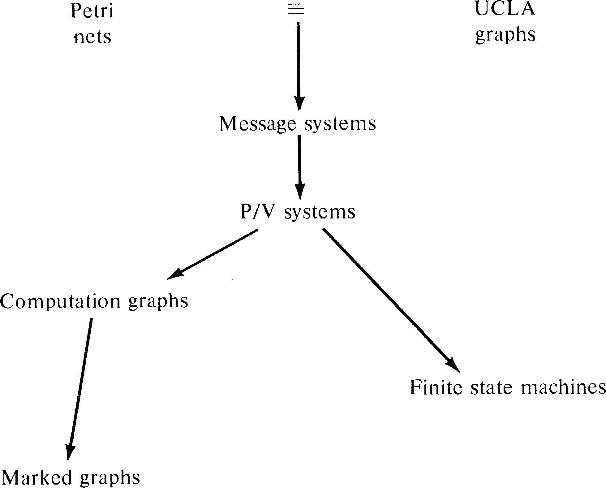
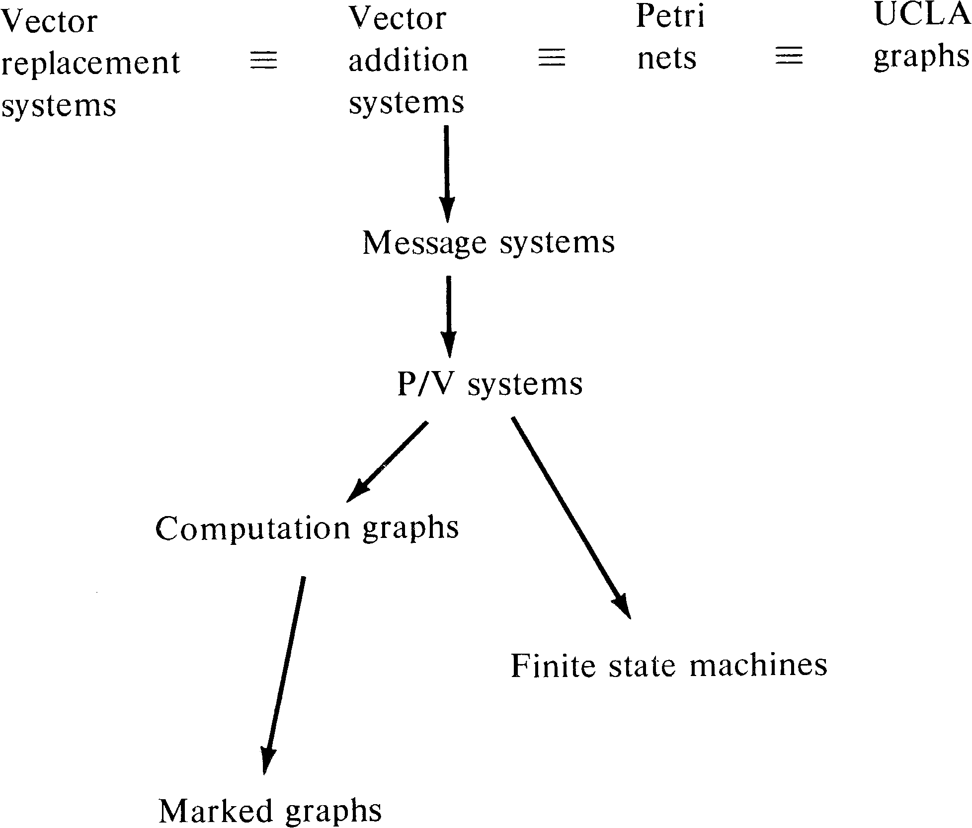
We have already seen in Sections 3.3.1 and 7.4.1 that finite state machines can be transformed easily into Petri nets. Finite state machines have been used by several researchers as a model of parallel computation. Bredt [1970b] defined a model based on computer hardware. Each processor is modeled as a finite state machine with input and output lines which connect a processor to other processors. The state of each input and output line is either 0 or 1. Since every output line for one processor is an input line for another processor and there are a finite number of processors and a finite number of lines each with a finite state, the entire system is finite state.
Gilbert and Chandler [1972] used a model with common memory
rather than communication lines. This means that their
model is directed more toward modeling computer software
processes with shared memory rather than the hardware model
of Bredt but is nonetheless a finite state model and
hence included in the Petri net model.
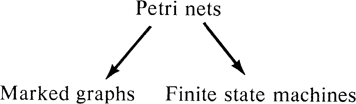
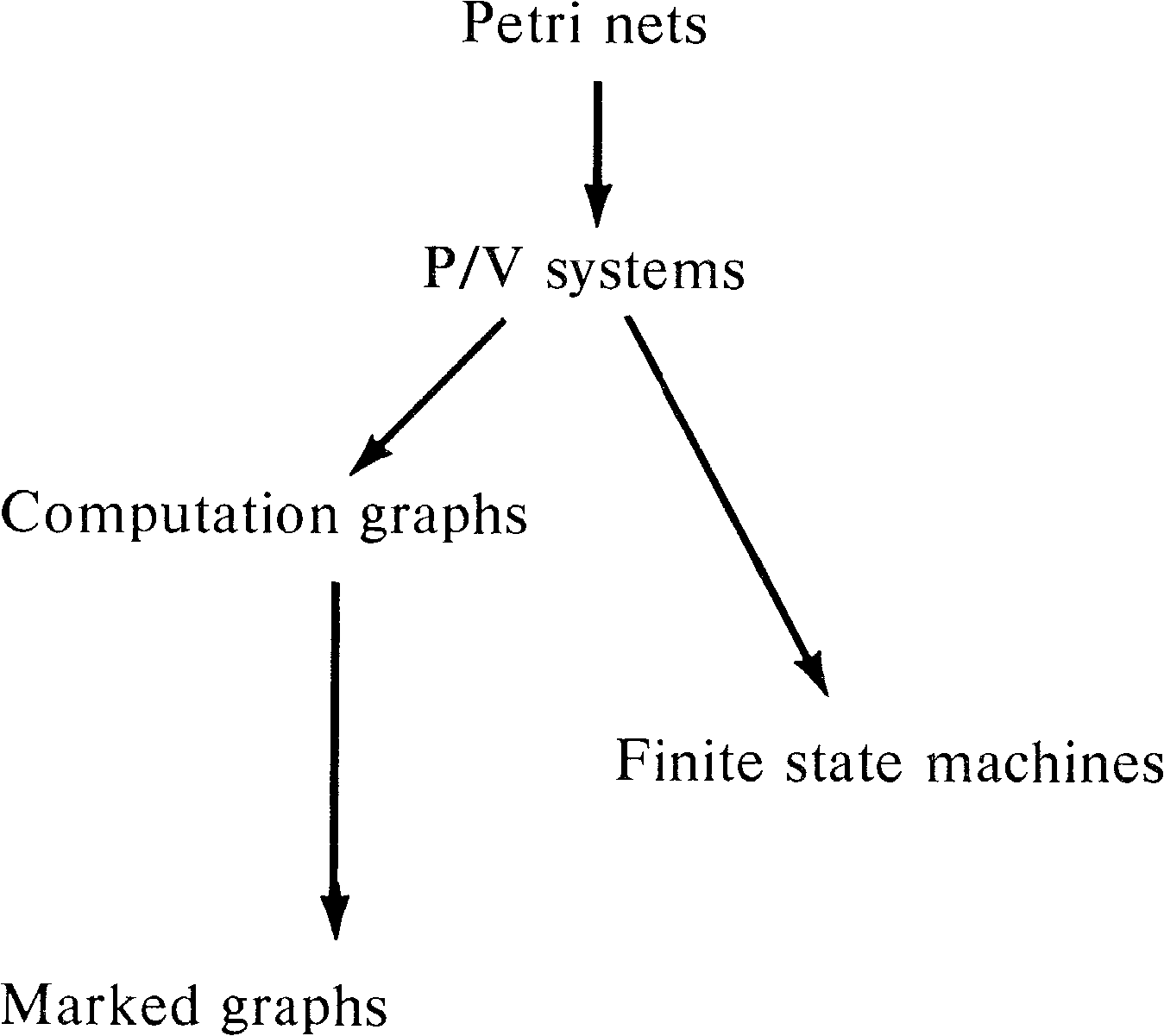
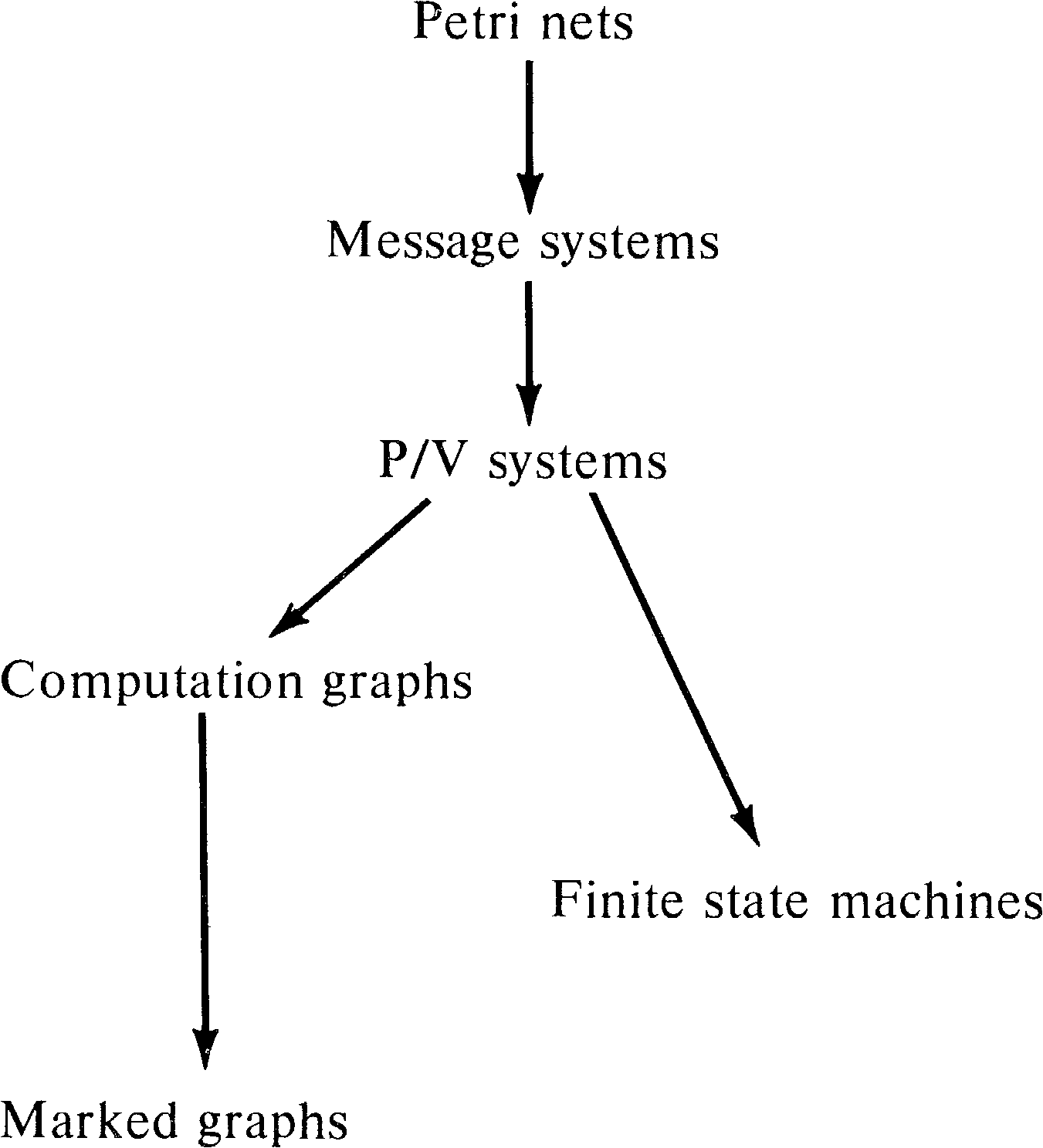
8.2. Marked Graphs
Marked graphs have been discussed in Section 7.4.2.
As a subclass of Petri nets, marked graphs are obviously of
more limited modeling power than Petri nets. Marked graphs
are not directly comparable to finite state machines but
rather seem to be duals. This provides us with the
relationships in Figure 8.1 among Petri nets, finite state
machines, and marked graphs.
One of the earliest models of parallel computation was the computation graph model [Karp and Miller 1966]. This model was mainly designed to represent the execution of programs evaluating arithmetic expressions in parallel.
A computation graph G is defined by a directed graph
G = ( V, A ), where
| V | = | { v1, v2, …, vn } is a set of vertices |
| A | = | { a1, a2, …, am } is a set of arcs |
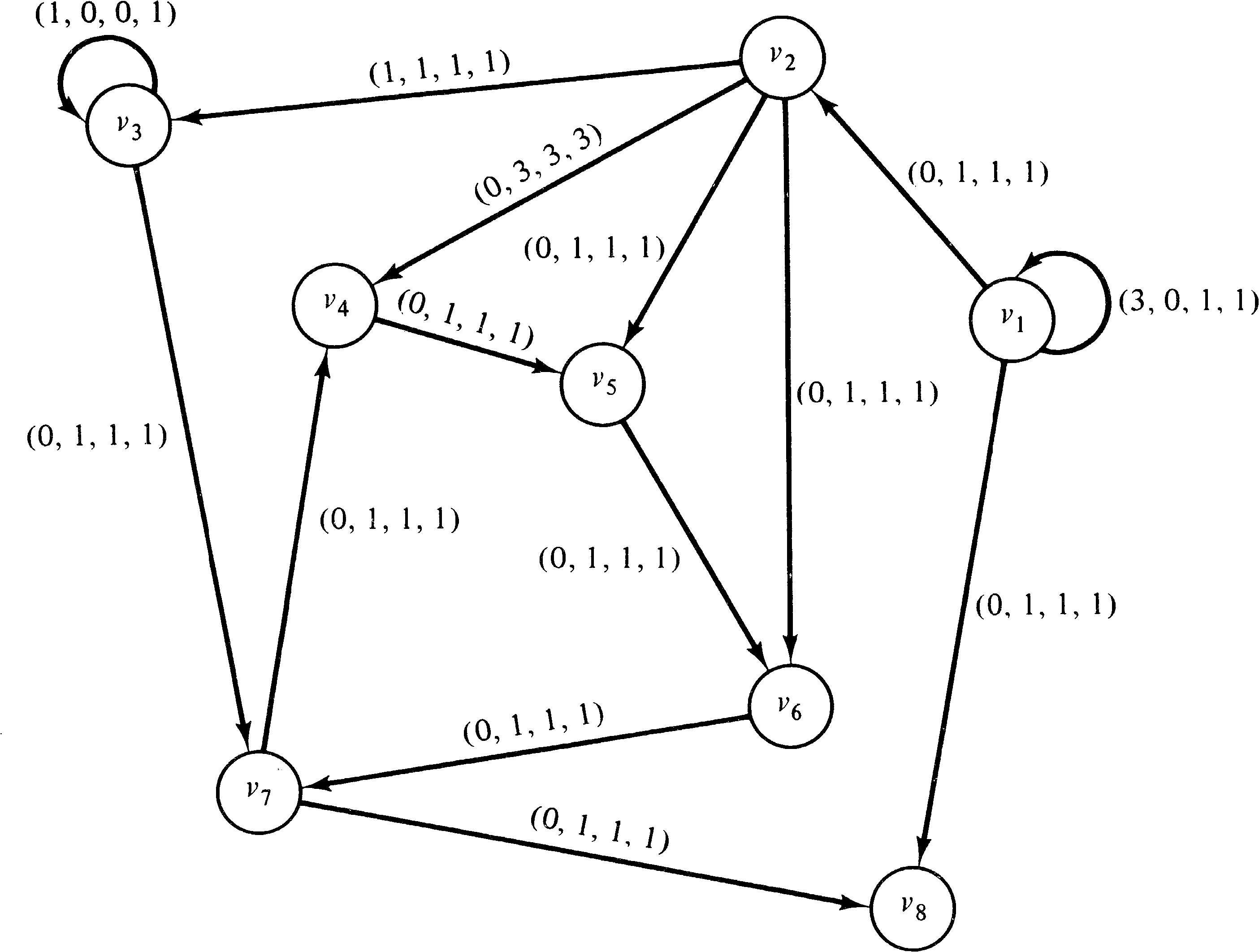
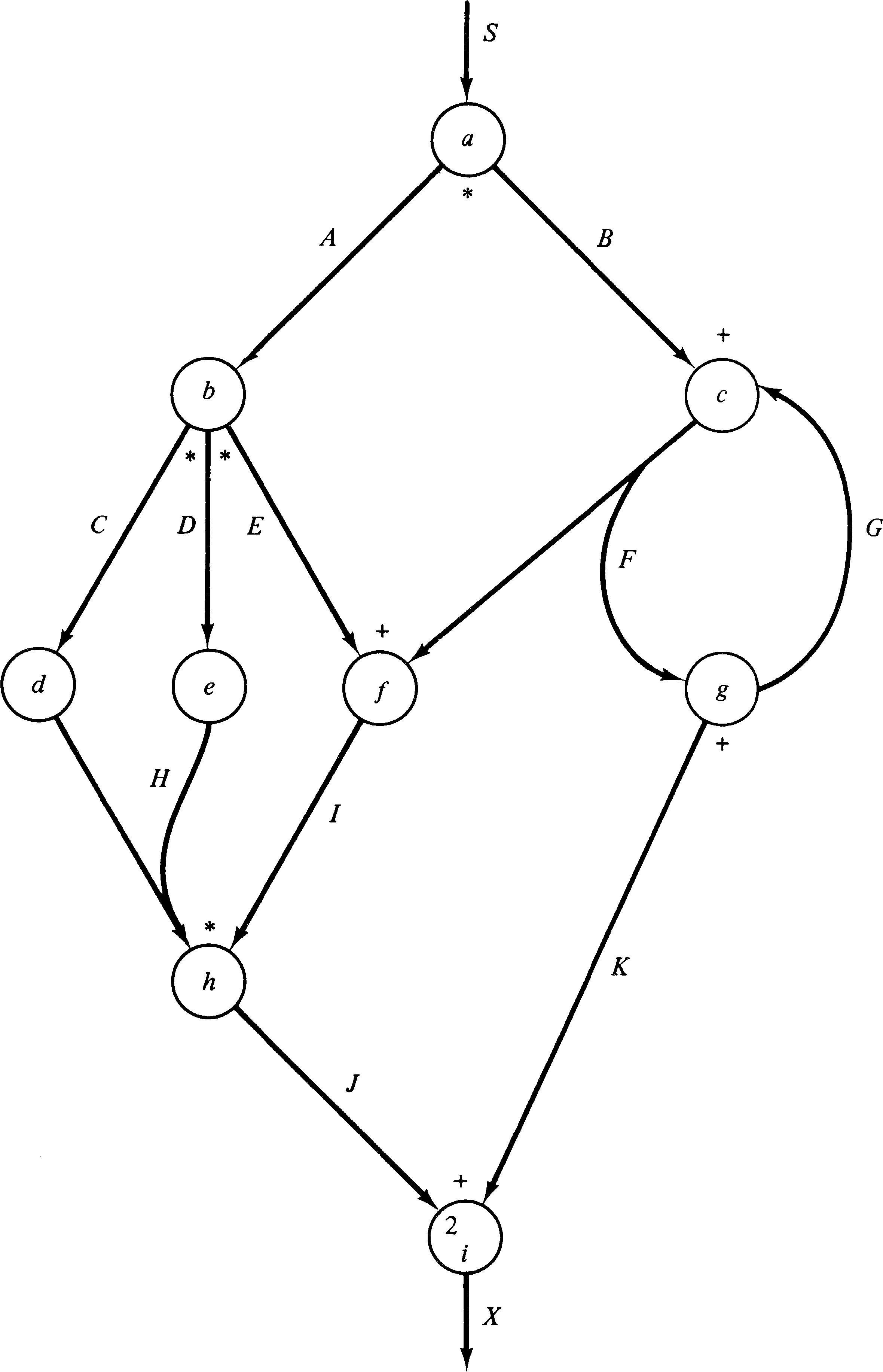
Figure 8.2 is an example computation graph. In the initial
state, the node v1 is enabled, since it has one
input and this input has three data items in its queue. When
v1 executes it removes one data item from this
queue and upon completion puts one data item on the arc from
v1 to v2 and one on the arc from
v1 to v8. In this new state either
v1 or v2 can execute since both have
enough data items in their input queues to satisfy their
thresholds.
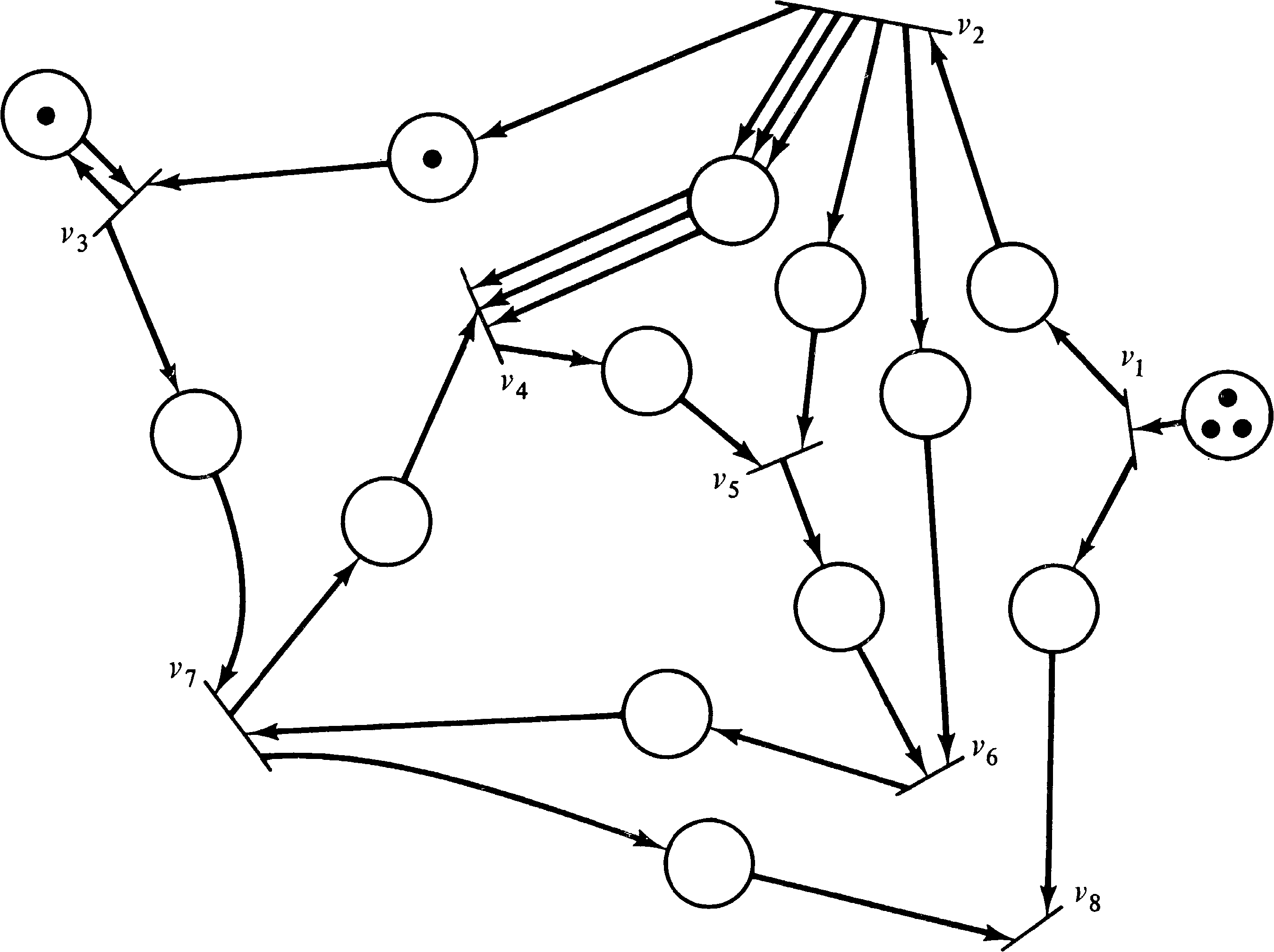
A computation graph is easily modeled as a Petri net. Each arc is represented by a place, and each node of the computation graph becomes a transition. The transition corresponding to node vk has Tj, k input arcs from the place representing an arc from vj to vk. This assures that the transition is enabled only if the threshold is met. However, when the transition fires it can only remove Wj, k of these tokens, so Tj, k − Wj, k arcs are directed back from transition vk to the place representing the arc from vj to vk. In addition Vk, r tokens are put into the places representing arcs from node vk to node vr. The initial marking is determined from the Ij, k as would be expected.
Figure 8.3 shows the Petri net constructed by this means
from the computation graph of Figure 8.2.
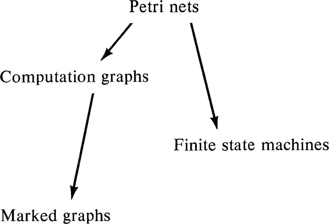
A little thought shows that marked graphs can be modeled as computation graphs with Tj, k = Wj, k for all nodes vj and vk. However, computation graphs are more powerful than marked graphs because of the ability to have Tj, k > Wj, k.
On the other hand, computation graphs and finite state
machines are incomparable, as are marked graphs and finite
state machines. Computation graphs cannot model decisions
or conditional execution -- the same limitation that marked
graphs have. Thus, our hierarchy of models at this point is
as shown in Figure 8.4.
Karp and Miller [1966] thoroughly investigated computation
graphs, especially concerning the problems of liveness and
safeness. Actually, Karp and Miller were interested in
assuring that a computation graph would terminate and so
determined the conditions for a computation graph to
terminate (i.e., to not be live). Since the arcs
(places) represented queues of data, Karp and Miller's
investigation of boundedness was aimed at determining the
maximum queue length. These differences in notation and
motivation as well as the difference in model definition
between computation graphs and marked graphs has meant that
no one has tried to relate the results and algorithms of
Karp and Miller [1966] on computation graphs with the work
on marked graphs [Commoner et al. 1971].
8.4. P/V Systems
P and V operations on semaphores were first introduced by Dijkstra [1968] to aid in solving synchronization problems in systems of parallel processes. As such they can be used to model synchronization and communication in the same way as Petri nets. Patil used this approach when he defined the cigarette smokers' problem to show the limitations of systems which can use only P and V operations between processes. P/V systems are nonetheless quite popular, and the computing science literature abounds with discussions or applications of these operations, for example, [Liskov 1972; Brinch Hansen 1973].
Section 3.4.8 showed that P and V operations can be modeled using Petri nets, and Patil's proof [Patil 1971] shows that the inclusion is proper: There are problems (the cigarette smokers' problem, for example) which can be solved with Petri nets but not with P and V operations only. However, P/V systems are powerful enough to include both computation graph models [Lipton and Snyder 1974] and finite state machine models.
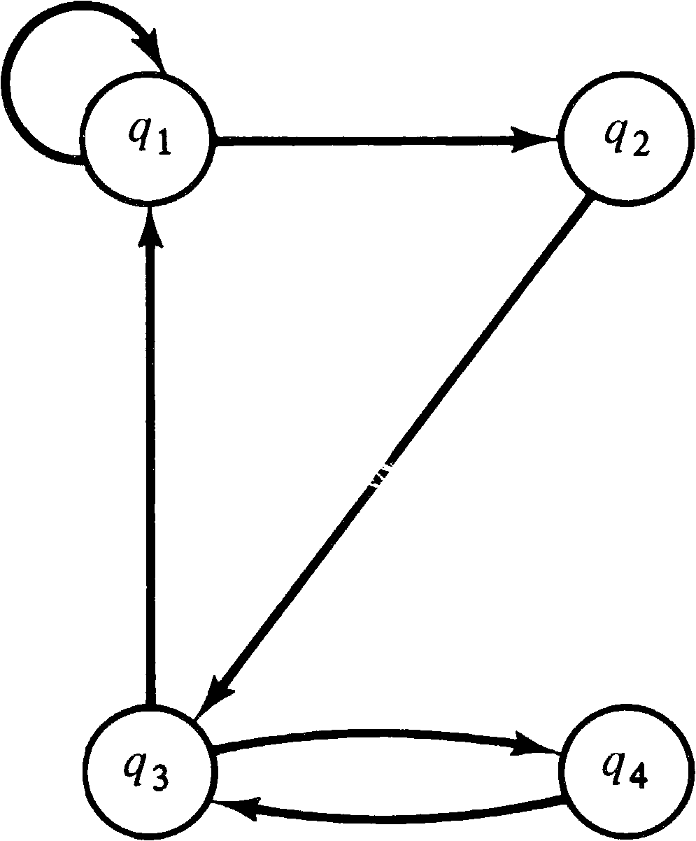
To convert a finite state machine into a P/V system, we use
a separate process to model each state of the finite state
machine. One semaphore is associated with each state. Let
Q = { q1, q2, …, qn } be
the set of states and δ: Q ⨯ Σ → Q
be the next state function, with a set of actions Σ .
Associate with state qi a semaphore
Si and a process. The process first executes a
P (Si ) . Generally it will wait here until the
state of the finite state machine becomes
qi. After the P (Si ), the process
arbitrarily picks any σ ∈ Σ for which
δ ( qi, σ ) is defined and executes
a V ( Sj ), where
qj = δ ( qi, σ ) .
Then this process
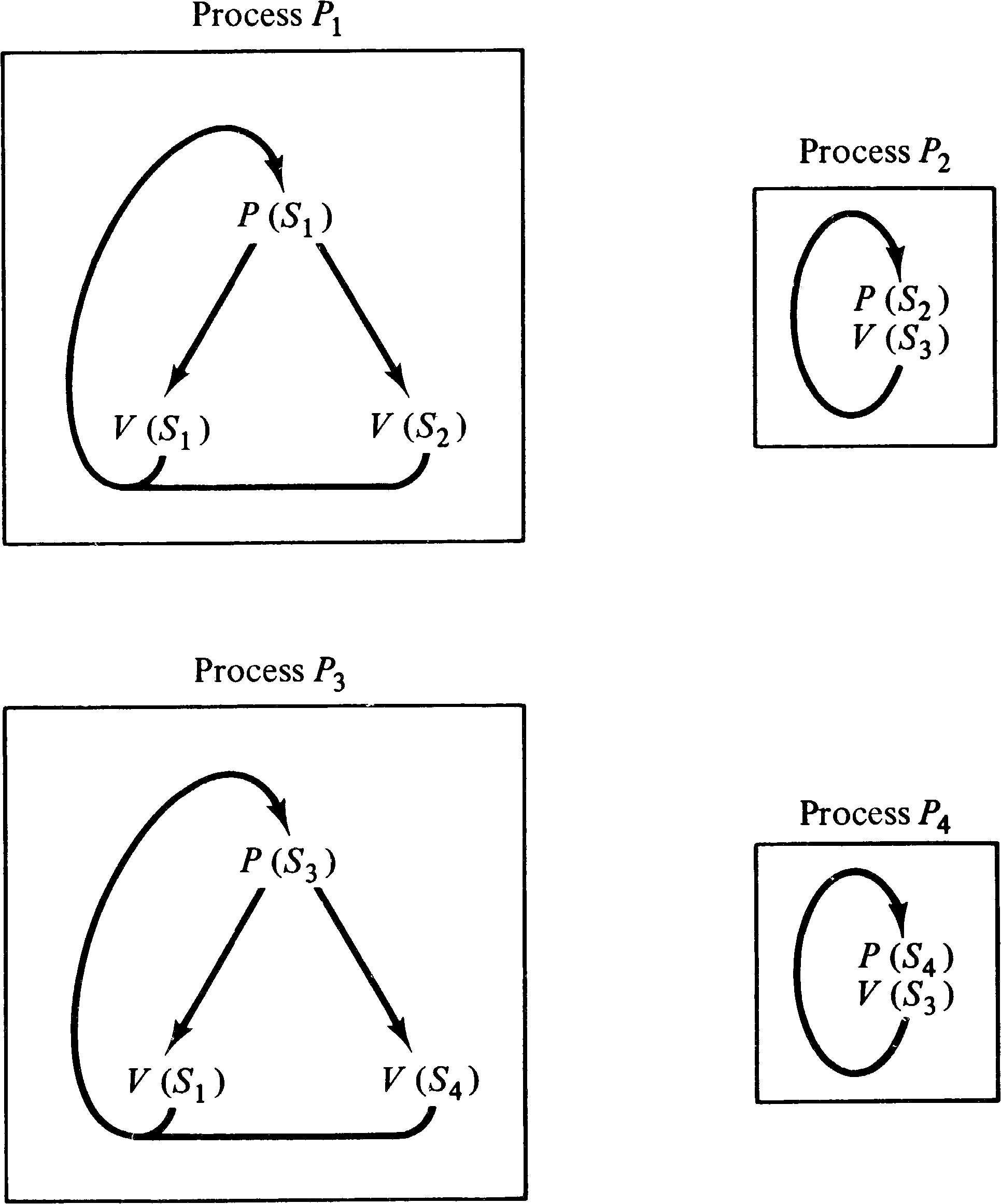
loops back to its P (Si ) . Figure 8.5 illustrates
this conversion on the finite state machine of Figure 8.6.
The semaphores are initially zero, except for the semaphore
for the start state, which is initialized to one.
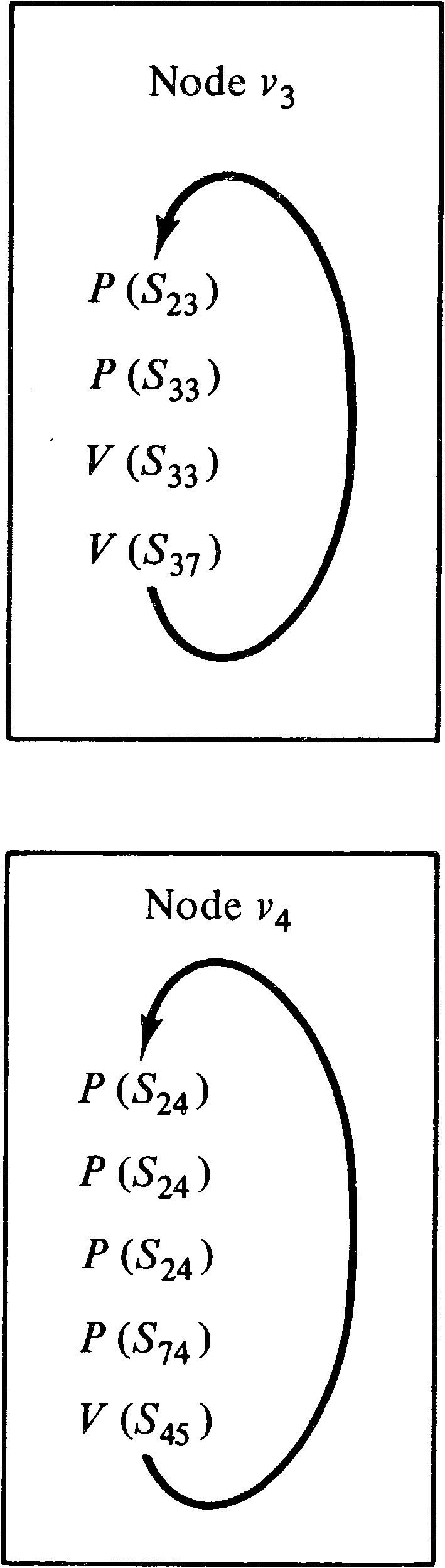
To convert a computation graph into a P/V system, we associate a semaphore Sj, k with each arc ( vj, vk ) in the graph. The value of the semaphore will be the number of data items waiting on the queue for that arc. Thus, initially the value of semaphore Sj, k is Ij, k. A process is created for every node in the computation graph. The process for node vk first executes Tj, k P operations on semaphore Sj, k for all arcs ( vj, vk ) directed into vk. This assures that each queue has at least Tj, k data items in it. Then, since each P operation decremented the semaphore and the correct effect is only to decrease Sj, k by Wj, k, we execute Tj, k − Wj, k V operations on Sj, k to restore the correct value of Sj, k. Now we complete the process for node vk by executing Vk, r V operations on semaphore Sk, r for each arc ( vk, vr ) directed out of node vk.
This conversion is illustrated in Figure 8.7 for the nodes
v3 and v4 of the computation graph of Figure 8.2.
Notice that the computation graph could test and input from several sources at once, while P/V systems can only test and input from several sources by a sequence of tests and inputs from single sources. The inability to test and input from several sources simultaneously is the key to Patil's proof of the limitations of P/V systems, the problem being that another process may grab the second source while you grab the first, leading to a deadlock. This is not a problem with computation graphs because the sources are not shared between processors -- no two nodes ever share an input arc. This point is crucial to constructing a P/V system which will not deadlock (terminate) unless the corresponding computation graph also terminates.
The addition of P/V systems to our hierarchy of models gives
us Figure 8.8.
Systems in which processes communicate via P and V operations on semaphores may be doing so for lack of a better communication mechanism. One suggestion for a better mechanism is messages. A message system is a collection of processes which communicate by messages. Two operations on messages are possible: send and receive. Sending a message is similar to a V operation; receiving a message is similar to a P operation. If no message is present when a receive is executed, the receiver waits until a message is sent.
This mechanism has been used as the basis of a modeling scheme by Riddle [1972]. This model would seem most appropriate for modeling computer network protocols. Riddle considers a (finite) set of processes which communicate by means of messages. Messages are sent to and requested from special processes called link processes (mailboxes). Link processes provide what is essentially a bag of messages which have been sent and not yet received or requests for messages from receives which have been made but not yet satisfied. The other processes of the system are called program processes and are represented in the program process modeling language (PPML).
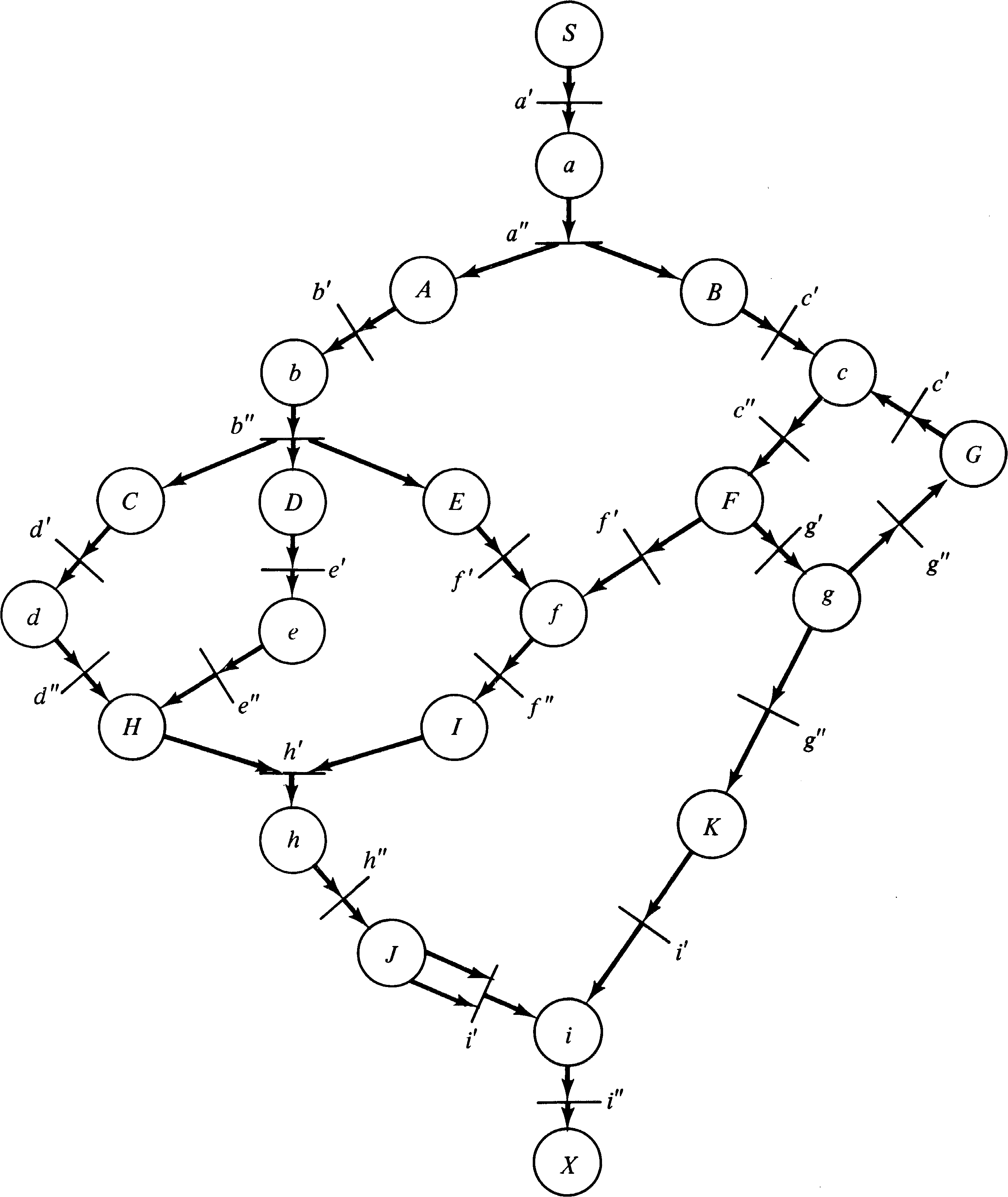
An example system of three processes is given in Figure 8.9.
As can be seen, the PPML description of the processes is
essentially a schema. Only the transmission activity of
messages in the system is of interest. Messages are abstract
items whose only characteristic is a type. There may only
be a finite number of types of messages in a system.
Messages are sent from and received into a message buffer in
each process. There is only one buffer per process. The
statements in PPML are
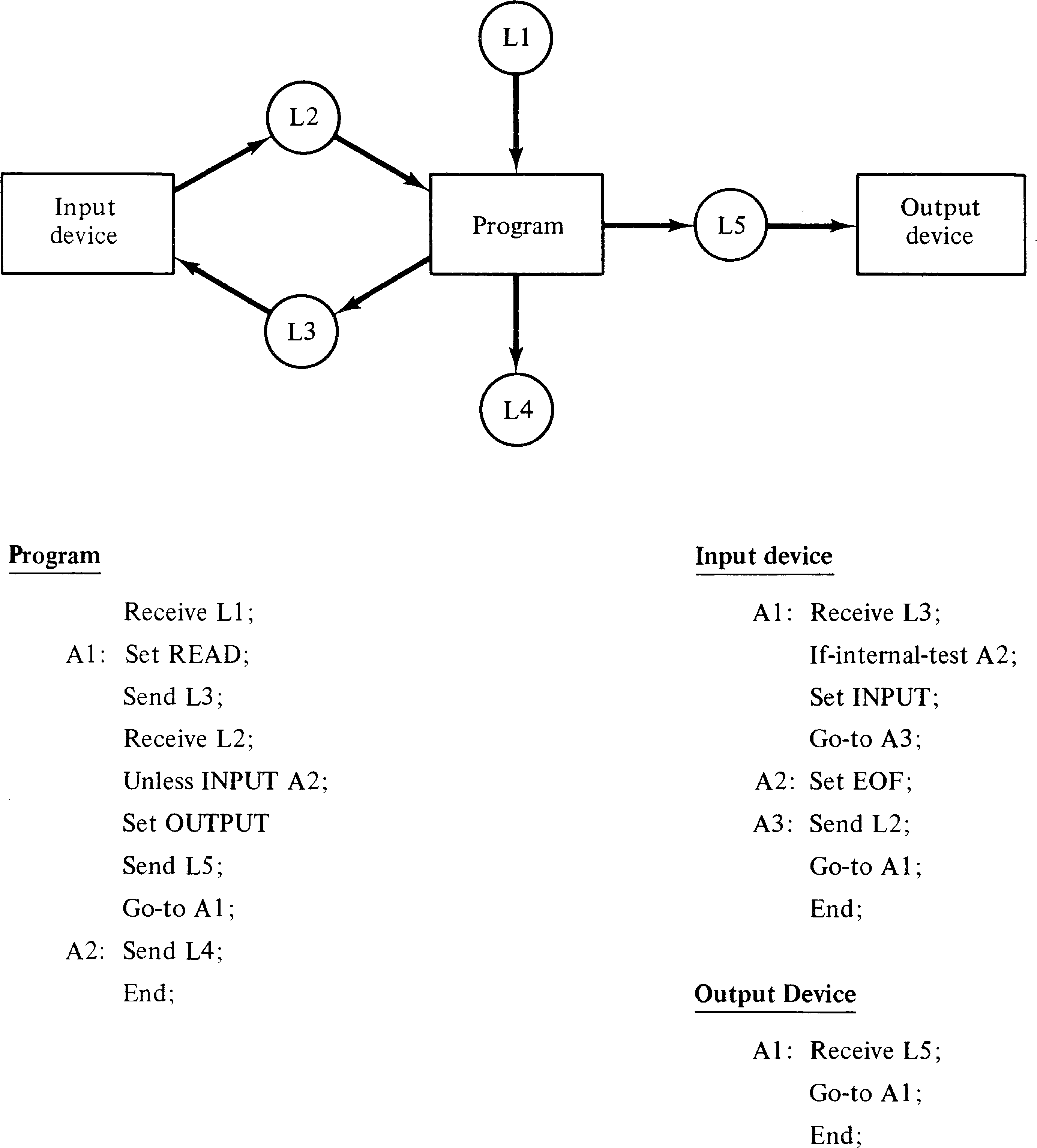
The PPML system models a set of parallel processes. Each process is started at the beginning of its program and executes its program until it encounters an end statement. Riddle shows how to construct a message transfer expression which represents the possible flow of messages in the system and uses this expression to examine the structure of the system for correct operation. This message transfer expression is used for the same purpose as the language of a Petri net. Therefore, we show how a PPML description of a system of processes can be converted into a Petri net whose language is equal to the message transfer expression of Riddle's analysis. This conversion ignores the execution of the individual statements of the PPML descriptions, although with only minor modification these could also be represented in the Petri net language.
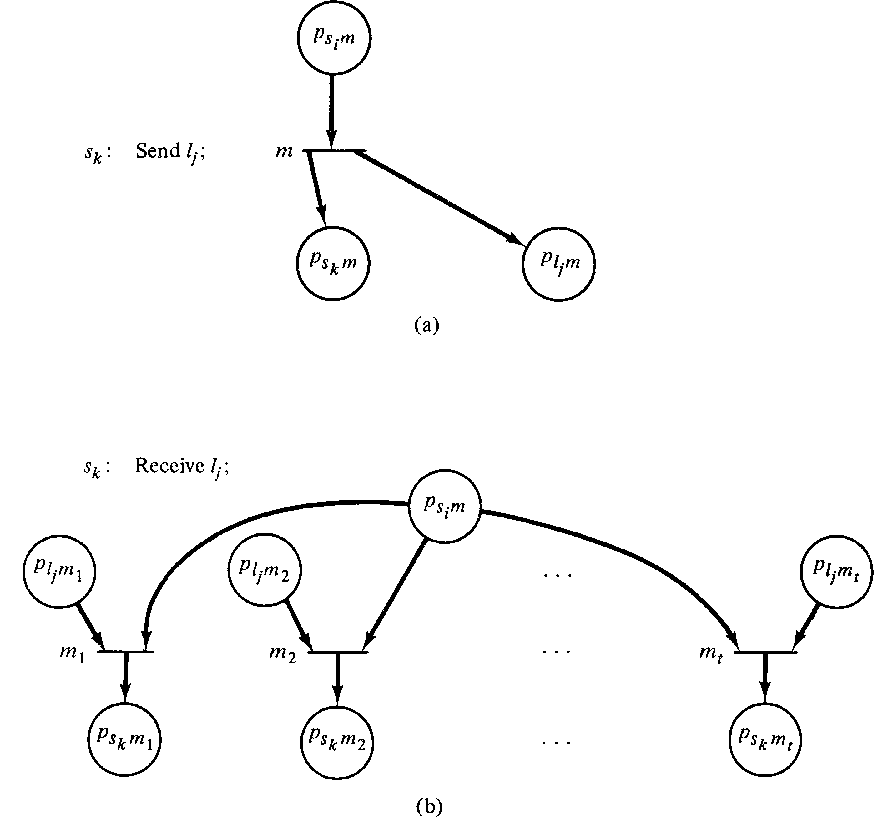
To model a process as a Petri net, we use one token per process as a program counter. The presence of a message in a link process is also represented by a token. Since the messages are identified by type, it is necessary to model each type of message in a link process by a separate place. A very important property of PPML systems is that the number of message types is finite. Each program process is also finite. Only the queueing of messages involves a potentially unbounded amount of storage. Thus the ability to model the link processes and to represent the send and receive statements correctly is the most important aspect of the transformation from a PPML description to a Petri net. By modeling the link processes by a set of places (one for each message type), we can represent a send statement by a transition which places a token in the place representing the appropriate link process and message type. The receive statement merely removes a token from any one of the places of a link process. The particular place which supplies the token determines the type of the message which was received. This information can be used in any subsequent unless statement.
The only symbols in a message transfer expression are the
message types for the messages which are sent to or received
from a link process. Since every transition in a Petri net
results in a symbol in the Petri net language for that Petri
net, only the send and receive statements in a
PPML system can be modeled. Thus there are two kinds of
places in the Petri net. One kind of place, labeled
pli, mj, acts as a
counter of the number of messages of type mj
in link process li. The other kind of place
represents the send and receive statements of
the PPML programs. Let the statements be uniquely labeled
s1, …, sr. We label the place
representing a statement si with a message
of type mj in the message buffer by
psi, mj. A token
in a place associated with a statement si
means that statement si has just been
executed. Figure 8.10 illustrates how a send and
receive statement at sk would be
modeled in the Petri net. In Figure 8.10, place
psi, m represents the place
associated with any statement which precedes the statement
sk.
It remains only to show that it is possible to determine
which statements can precede other statements in the PPML
program. Notice that we must consider each statement as a
pair consisting of a message type and a statement number,
since the same statement with different message types in the
message buffer will be modeled differently in the Petri net.
The most obvious method to determine the predecessors of a
statement is to start at the beginning of each PPML program
with a special start statement (which will become the start
place) and follow the program description generating all
possible send and receive statements which can
follow this statement with their corresponding message
buffer contents. This process is repeated for all newly
reachable statements until all such send and
receive statements have been generated and their
successors identified. Since the number of statements in a
PPML description and the number of message types are finite,
only a finite number of statement/message-type pairs
will be generated. This procedure is similar to the
characteristic equations used by Riddle [1972] to construct
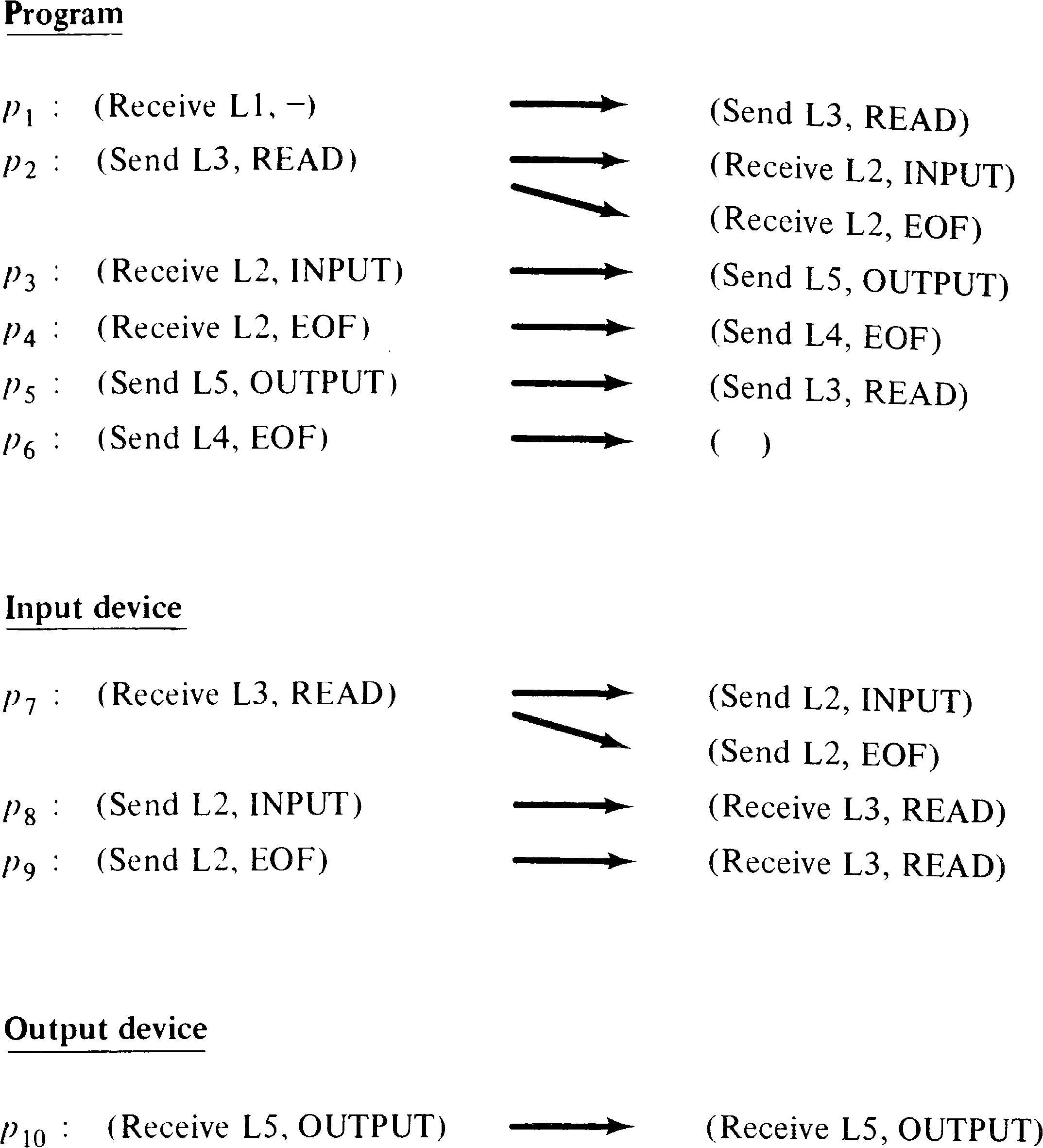
the message transfer expression. Figure 8.11 lists the
statements and their possible successors for the PPML system
of Figure 8.9.
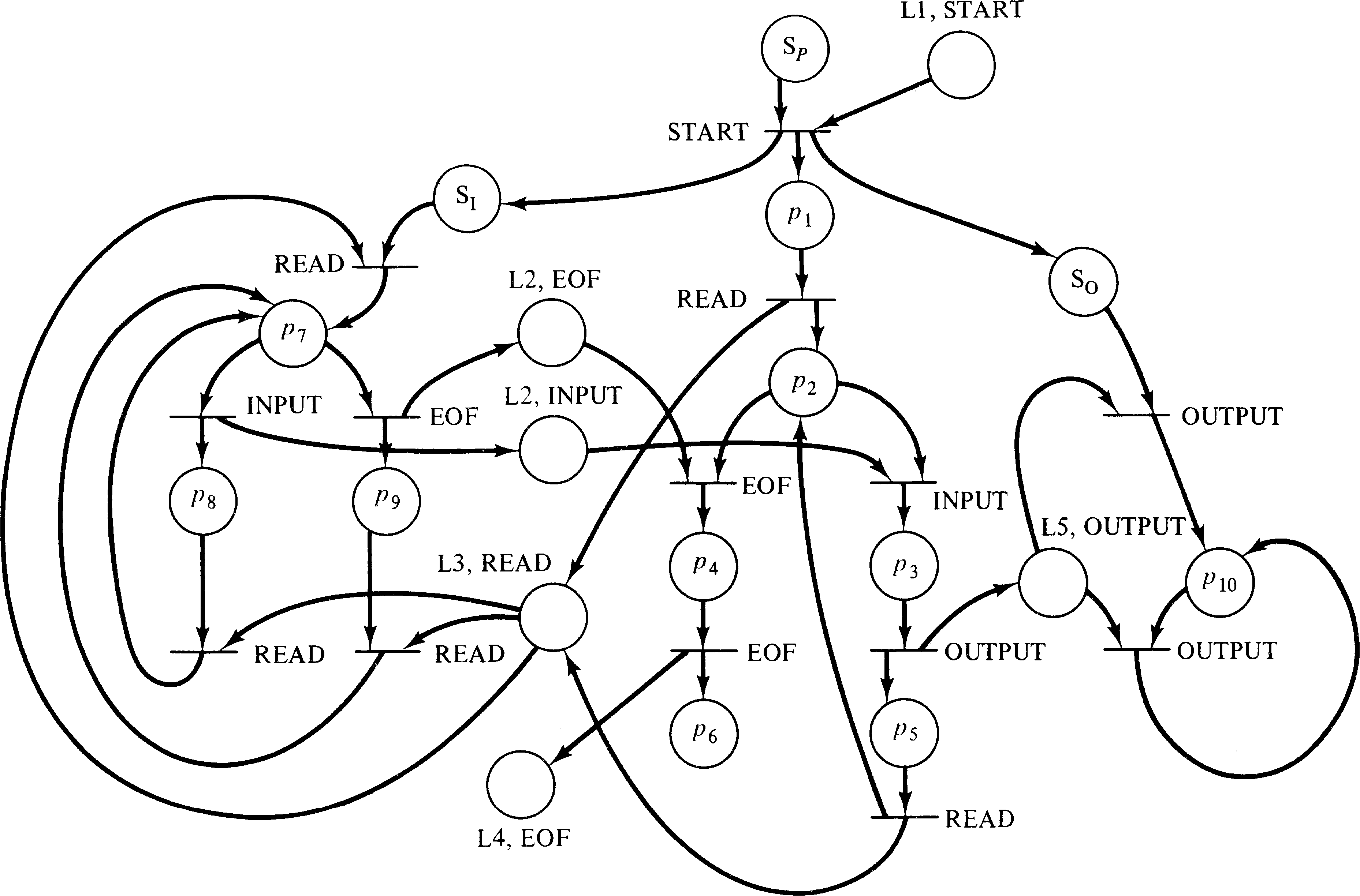
Once the successors of a statement have been determined,
this information can be used to identify the possible
predecessors of a statement and hence to construct a Petri
net which is equivalent to the PPML system by use of
transitions such as given in Figure 8.10. A special start
place is the predecessor of the first statements of each of
the processes of the system. Figure 8.12 transforms the PPML
system of Figure 8.9 into an equivalent Petri net.
This brief description of the transformation from message transmission systems to Petri nets shows that this model is included in the modeling power of the Petri net. It also shows that the set of message transfer expressions, considered as a class of languages, is a subset of the class of Petri net languages.
Since P/V systems can be modeled as message transmission systems with all messages being the same type, P/V systems are included in message transmission systems. It is fairly easy to construct a message system to solve the cigarette smokers' problem, however, so the inclusion of P/V systems in message systems is proper. Message systems, on the other hand, lack the ability to input from several sources simultaneously and so are not equivalent to Petri nets. One of two cases will occur in an attempt to model a transition with multiple inputs:
Riddle [1974] presents a transformation which suffers from case 1,
leading to spurious deadlocks. In either case, we see that message
systems cannot model arbitrary Petri nets (under our
constraints). This results in the hierarchy of Figure 8.13.
Petri nets are a graph model of parallel computation. Another graph model has been developed at the University of California at Los Angeles under the direction of Professor Estrin. This model is the complex bilogic graph model of computation (or UCLA graph model) [Baer 1968; Baer et al. 1970; Volansky 1970; Gostelow 1971; Cerf 1972]. In this model, systems are represented by a graph with complex directed arcs. A complex arc is an arc with (potentially) multiple sources and destinations.
Combinational logic controls the sequencing of operations at the nodes. If the input logic of a node is AND (*), tokens are needed on each input arc to enable an operation. For OR (+) logic, tokens are only needed on some one input arc. Execution of the node removes the enabling tokens on the input arcs and places tokens on the output arcs according to the output logic. For AND output logic, tokens are placed on all output arcs, while for OR logic, tokens are placed on any one output arc. The number of tokens involved for a given node-arc pair is the degree (or multiplicity) of that pair and may be any nonnegative integer.
Figure 8.14 is an example UCLA graph. Notice that some arcs
have multiple sources (tails) and destinations (heads).
Also notice that the logic of each arc-node pair is marked
on the graph as either * for AND logic or + for OR logic.
The degree of an arc is indicated by a small number where
the arc meets the node. The degree is omitted if it is one,
as is the logic when only one arc is the input to a node.
In the example node a can fire whenever arc S has
a token. When node a fires, it removes the
token from arc S and puts tokens on both arc A and arc B
(AND logic). Node g, on the other hand, will place a
token on either arc K or arc G (OR logic). Node i is
enabled whenever there are two tokens on arc J or one token
on arc K.
| V | = | { v1, v2, …, vr } is a set of vertices |
| A | = | { a1, a2, …, as } is a set of arcs |
| L | = | (L−, L+): V → { *, + } is the input(L−) and output(L+) logic mapping for each vertex |
| Q | = | (Q−, Q+): V ⨯ A → N is the input(Q−) and output(Q+) degree of each arc−vertex pair |
| S ∈ A is the start arc | ||
| F ∈ A is the final arc |
The transformation from a UCLA graph to a Petri net is
straightforward due to the similarity of the two systems.
Every arc in a UCLA graph is represented by a place in a
Petri net. In addition, we represent a node v by a
place pv and two transitions
tv′ and
tv′′ . The first transition
tv′ represents the initiation of
the operation associated with node v; the second
transition represents the termination of the
operation. This is sketched in Figure 8.15. (The modeling
of UCLA graph nodes by initiation and termination
transitions is not strictly necessary but is convenient.)
Figure 8.16 indicates how the input and output logic for
UCLA graphs is represented in an equivalent Petri net.
Degrees greater than 1 are modeled by multiple arcs
between places and transitions in the Petri net.
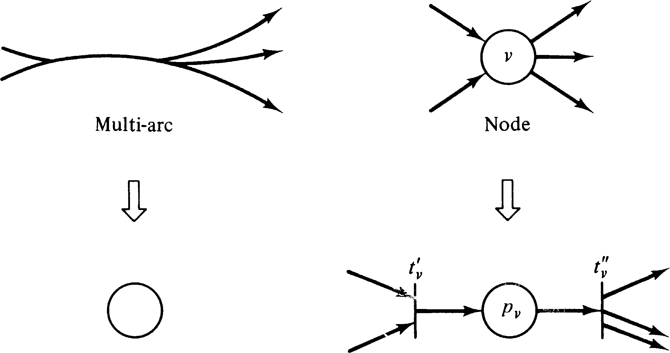
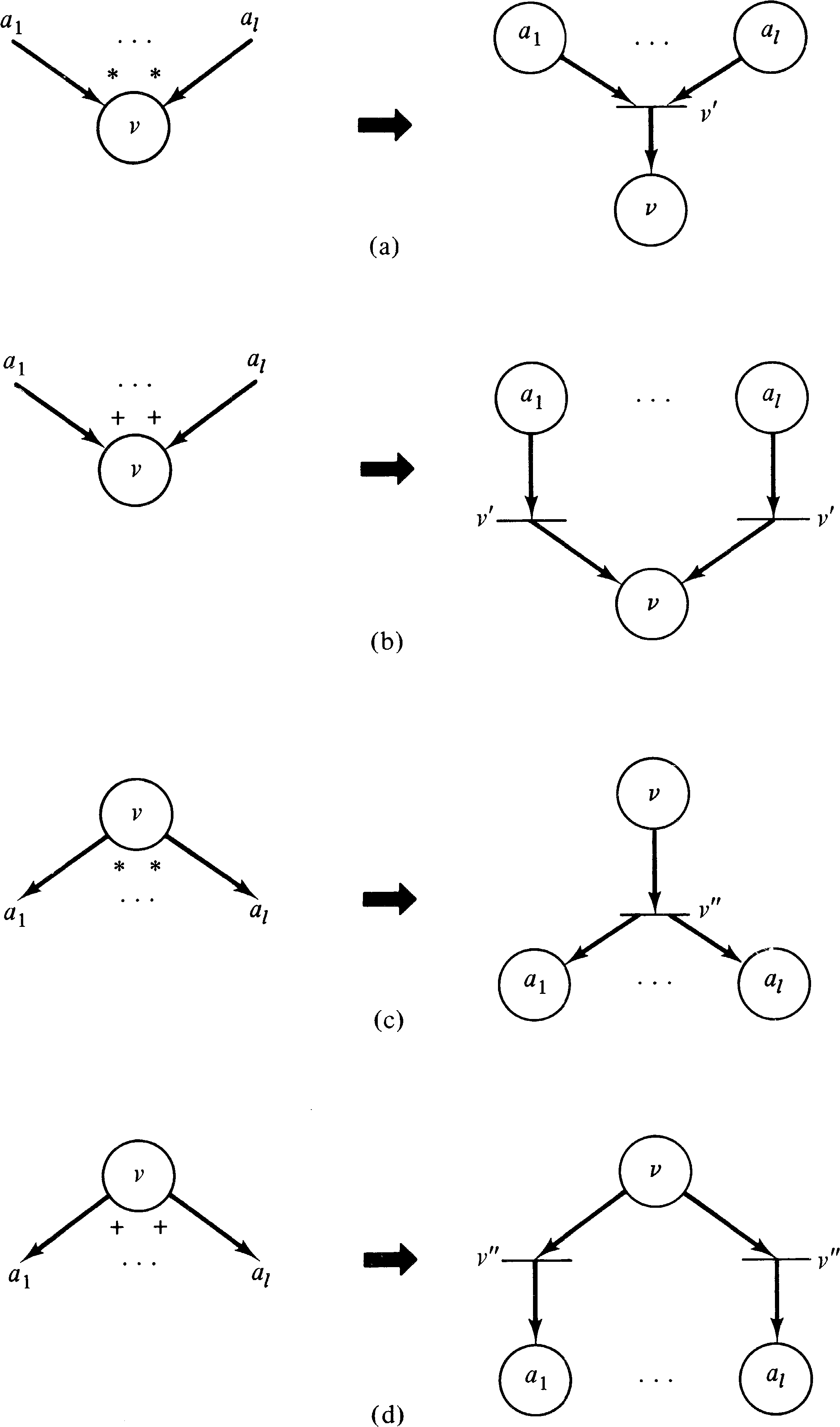
Figure 8.17 transforms the UCLA graph of Figure 8.14 into an
equivalent Petri net.
This transformation shows that the modeling power of UCLA
graphs is included in the modeling power of Petri nets. It
should be obvious that a Petri net can be converted into an
equivalent UCLA graph by representing places as UCLA graph
arcs and transitions as nodes with AND input and output
logic. Thus these two models are equivalent in modeling
power. Figure 8.18 shows the modified hierarchy of models.
If you have glanced at the bibliography you may have noticed that many of the references have titles referring not to Petri nets but to vector addition systems. Vector addition systems were introduced by Karp and Miller [1968] as a mathematical tool for analyzing systems of parallel processes. Because of their simple mathematical formulation, vector addition systems are typically used for formal proofs of properties of Petri nets or similar systems.
The reachability set of a vector addition system V is denoted R ( V ) and can be defined either recursively by
| k | ||||||
| x | = | s + | Σ | bij | ||
| j = 1 | ||||||
| r | ||||||
| s + | Σ | bij | ≥ | 0 | for all r, 0 ≤ r ≤ k | |
| j = 1 |
With these definitions, it is easy to see that vector addition systems and Petri nets are equivalent. Given a Petri net, we can construct a vector addition system whose start vector s is the initial marking, with one basis vector for each transition. The n components of the vectors of the vector addition system correspond to the markings of the n places of the Petri net, or in the case of the basis vectors to the change in marking resulting from firing the associated transition.
Similarly, a vector addition system can be converted into an
equivalent Petri net, using places for the components of the
vectors and transitions to represent basis vectors. Figure
8.19 illustrates the equivalence of these two models.
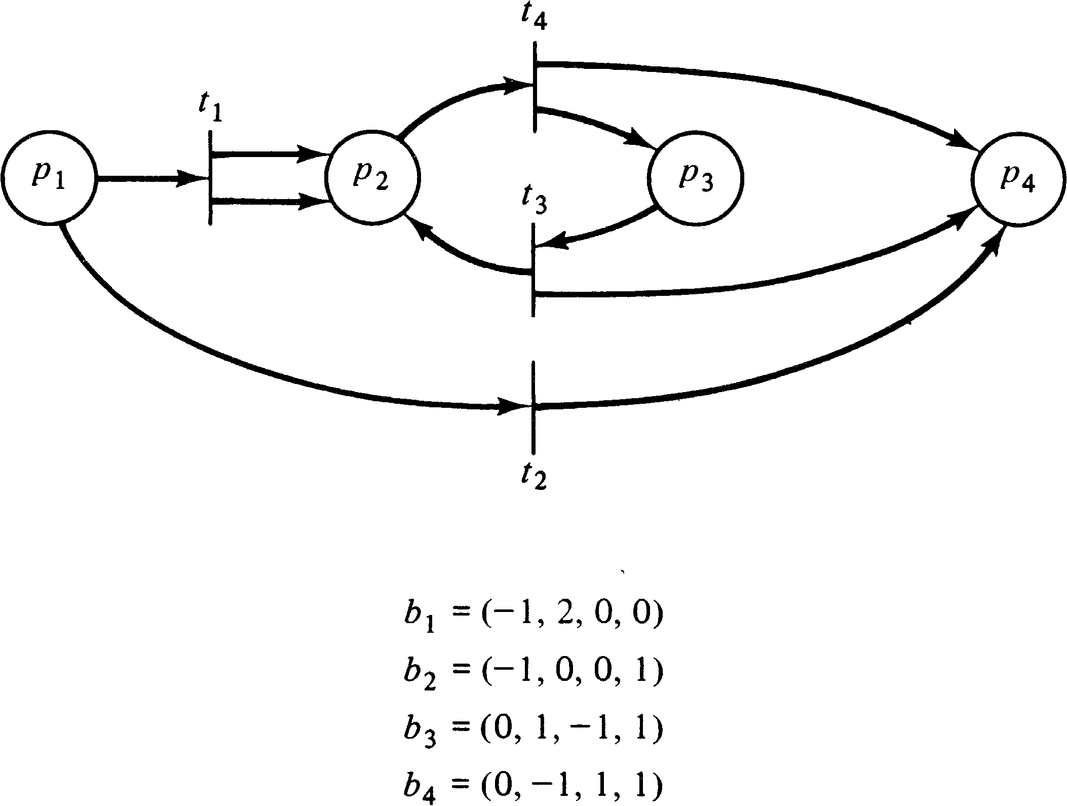
In fact, vector addition systems are equivalent to self-loop-free Petri nets. Remember that with a self-loop, the change is zero, but the number of tokens in the self-loop place must be nonzero. This does not diminish the power of vector addition systems, since we have seen (in Section 5.3) that self-loop-free Petri nets are equivalent to general Petri nets. However, to more directly model Petri nets with self-loops in a vector addition system-like model, Keller has defined vector replacement systems [Keller 1972].
The Ui vectors are called test vectors. The reachability set is redefined such that s is in the reachability set, and if x is in the reachability set and x + Ui ≥ 0, then x + Vi is in the reachability set.
The vector replacement system model explicitly separates the test for enabling a transition from the action of firing the transition. The equivalence of vector replacement systems to (general) Petri nets is obvious.
Adding vector addition systems and vector replacement
systems to our hierarchy yields Figure 8.20. The importance
of vector addition and replacement systems stems from their
concise mathematical definition and the usefulness of this
definition in proofs of the mathematical properties of
systems.
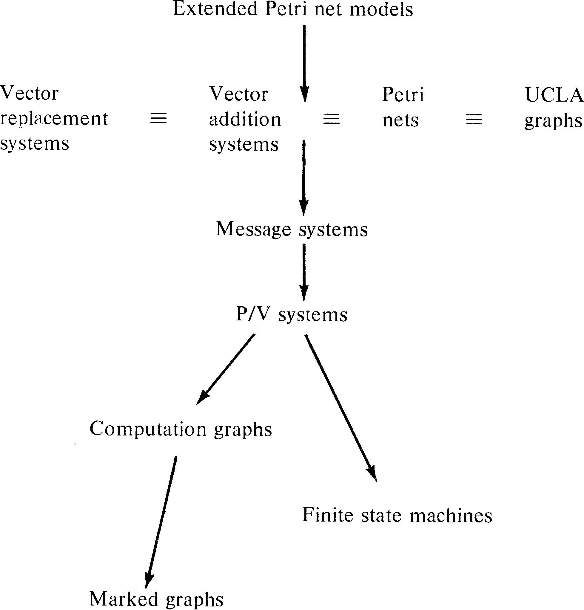
As a last addition to our hierarchy, we again mention the
extended Petri net models studied in Chapter 7: Petri nets
with constraints, exclusive-OR transitions, switches,
inhibitor arcs, priorities, or times. We have seen that all
of these models are equivalent to Turing machines. Thus
these models properly include Petri net models. Our final
hierarchy of models is shown in Figure 8.21.
The studies by Peterson and Bredt [1974], Agerwala [1974b], and Lipton et al. [1974] should be read first, since these are the most directly related works. Also read the surveys by Bredt [1970a] and Baer [1973a] and the work of Miller [1973; 1974]. The references in these papers will lead to the original work on the individual models.
Riddle's model [Riddle 1972] would appear to be the best for
modeling large software systems and deserves detailed study.
8.10. Topics for Further Study
| Home | Comments? |